Research Projects

In the third and the current step, we develop this approach further and apply a self-consistent convection model instead of random forcing. We include rotation and a polytropic stratification for the convection zone and an isothermal stratification for the corona. A large-scale magnetic field is generated self-consistently by the convective dynamo action underneath the surface.
In some simulations, we find ejections, which are similar the ones we found in earlier work (Warnecke et al. 2012), see Figure 3, where the averaged current helicity density, the magnetic field and the density is plotted for a convective driven ejection.
Coronal Mass Ejections Driven By Dynamo Action
Background information:
-------------------------
The Sun sheds plasma to the interstellar space via coronal mass ejections (CMEs). These ejections are driven by strong magnetic fields inside the Sun. Due to the high conductivity the magnetic field lines in the Sun are frozen in the plasma, known as the Alfven's theorem. Depending on the plasma beta, which is the ratio between the magnetic and the thermal pressure, the magnetic field is either dragged by the plasma motions or the magnetic field leads the motions of the plasma. In the convection zone and in the photosphere the first is the case, with exception of strong magnetic field regions, like sunspots and flux tubes. In the corona the plasma beta is less than unity and therefore magnetic field can transport plasma from lower to upper regions. In CMEs, magnetic field lines reconnect and dissipation of large amount of energy to Joule heating, which then drives the ejection of plasma outwards. In this context CMEs are also often called plasmoidal ejections, where the reconnection is described by an X-point. The ejected plasma reaches velocities which are higher than the escape speed of the Sun and enters the interplanetary space.
Some of these CMEs can hit the Earth and have a deep impact. They can cause the failure of power grids, distorting GPS signals and can also damage the microelectronics on space-craft orbiting the Earth. Additionally CMEs and connected events like flares can danger human missions to Mars or Moon.
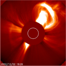
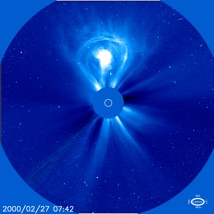
Coronal Mass Ejections (CME)observed by LASCO@ SOHO
There has been significant progress in the study of CMEs in recent years. In addition to improved observations from spacecrafts like SDO or STEREO, there have also been major advances in the field of numerical modeling of CME events. However, till now, the origin and formation of CMEs are not clearly understood. CMEs mostly happen above an active region, i.e. a region on the solar surface with strong magnetic fields. These strong magnetic field in the Sun are generated by a dynamo within the convection zone. Even though, there are different opinions on the type of dynamo in the scientific community, the existence of a solar dynamo, which generates the strong magnetic field structures i.e. sunspots and the global 22 years variability is well established. However, currently most of the CME models describe the formation and evolution not entirely self-consistently and as single events. The models are initialized with a prescribed magnetic field and the velocity pattern at the surface of the Sun evolves by shearing and twisting the magnetic field at its footpoints at the surface, see e.g. Antiochos et al. (1999) and Török & Kliem (2003). The fact that the magnetic and velocity configuration on the surface is generated by a dynamo in the convection zone is neglected.
The two layer model:
------------------------------
We have developed a different approach to understand the formation of the magnetic and velocity configurations which drive the CMEs. In the last two years we have worked with a model, which includes the convection and the solar corona and therefore combines the subsurface dynamics with those above the surface, like Coronal mass ejections, in one domain. Starting with a very simplified model, we improved it in three steps so far and obtain at each step notable results. As a first step, we use a Cartesian coordinate system and the magnetic field is generated by a forced turbulent dynamo.
The fluid was isothermal and had a constant density in the upper part, which mimics the solar corona. However, we found recurrent plasmoid ejections, even though we neglect effects like magnetic buoyancy (Warnecke & Brandenburg, 2010), see Figure 1, where the time series of the magnetic field line is plotted during the evolution of one ejection event.
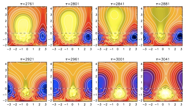
Figure 1: Time series of the formation of a plasmoid ejection. Contours of <Ax>x are shown together with a color-scale representation of <Bx>x ; dark blue stands for negative and light yellow for positive values. The contours of <Ax>x correspond to field lines of <B>x in the yz plane. The dotted horizontal lines show the location of the surface at z = 0.
As a second step, we use a spherical coordinate system and include a moderate density stratification due to gravitation. The magnetic field is generated here also by a forced turbulent dynamo underneath the surface, but to mimic the effects of rotation of the Sun to the flow, the forcing has a different sign of kinetic helicity in each hemisphere. With this setup we obtain also recurrent plasmoid ejections, which have a similar shape as the observed three-part-structure in CMEs. This is clearly see in Figure 2, where the averaged current helicity density is plotted for such an event.
As an additional result we found equatorward migration of the magnetic field structures at the surface, which are similar to the observed migration of sunspots (Warnecke et al. 2011).
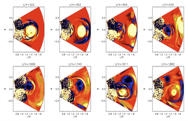
Figure 2: Time series of coronal ejections in spherical coordinates. The normalized current helicity, μ0R<J.B>Φ/<B2>Φt is in a color-scale representation for different times; dark blue stands for negative and light yellow for positive values. The magnetic and the fluid Reynolds number is 20.
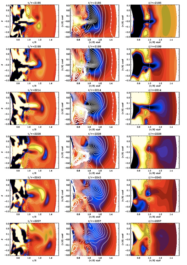
Figure 3: Time series of a coronal ejection zoomed into the region of the ejection near the equator ( θ=π/2). The dashed horizontal lines show the location of the surface at r = R. Left column: normalized current helicity, μ0R<J.B>Φ/<B2>Φt. Middle column: magnetic field, contours of r sinθ <AΦ>Φ are shown together with a color-scale representation of <BΦ>Φ. The contours of r sinθ <AΦ>Φ correspond to field lines of <B>Φ in the rθ plane, where solid lines represent clockwise magnetic field lines and the dashed ones counter-clockwise. Right column: density fluctuations <Δρ(t)>Φ = <ρ(t)>Φ − <ρ(t)>Φt. For all plots, the color-scale represents negative as dark blue and positive as light yellow.