 Instrumentation
and data reduction
Instrumentation
and data reduction
o 1.2.1 Dead-time & local gain correction
o 1.2.3 Geometrical distortion
o 1.2.4 Radiometric calibration
o 1.2.5 Wavelength calibration
o 1.2.6 Additional corrections
§ 1.2.6.1 Instrumental broadening
§ 1.2.6.2 Slit magnification and displacement
§
1.2.6.3 Long- and short-period instrumental
periodicities
1.1 The SUMER
SUMER is a powerful UV
instrument capable of making reliable measurements of bulk motions in the
chromosphere, TR and low corona with an accuracy better than 2 km s-1
(Wilhelm et al. 1997), with a spatial resolution of 1 arcsec (one arcsec at L1
corresponds to 715 km on the Sun) across the slit and 2 arcsec along the slit
(Lemaire et al. 1997). The basic characteristics, capabilities and operations
of
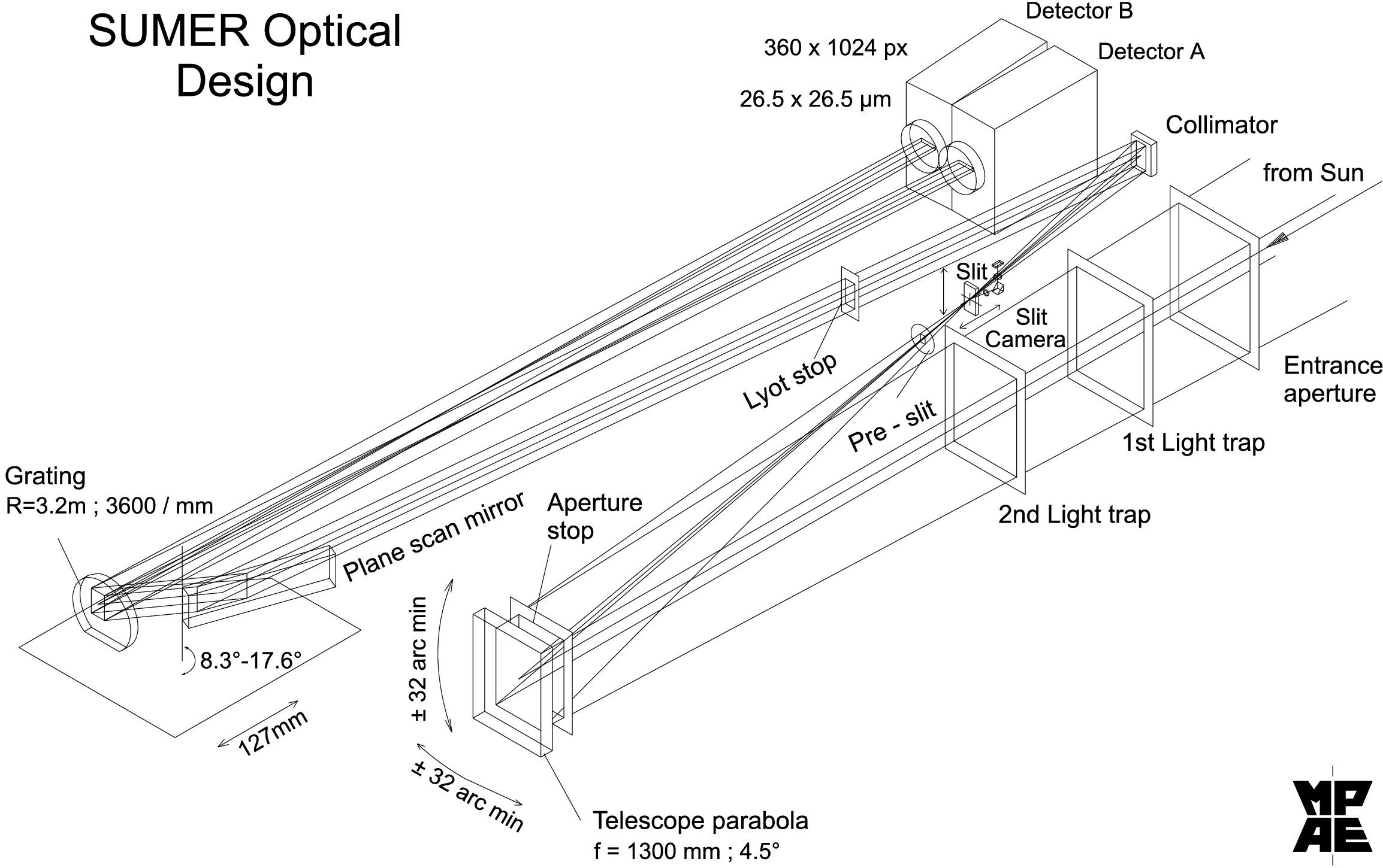
Figure
1.1: Optical layout of the
A brief summary of the
basic
Table 1.1:
|
Telescope: |
&xnbsp; |
|
|
|
&xnbsp; |
Focal length |
1302.77 mm at 75°C |
|
|
Equivalent f-number |
10.67 |
|
|
|
Plate scale in slit plane |
6.316 µm arcsec-1 |
|
|
|
Smallest
step sizes |
0.3763 arcsec |
||
|
&xnbsp; |
|
||
|
Slits: |
&xnbsp; |
|
|
|
&xnbsp; |
1 |
4.122 x 299.2 arcsec2 |
|
|
2 |
0.986 x 299.2 arcsec2 |
|
|
|
3 |
0.993 x119.6 arcsec2 (top) |
|
|
|
4 |
0.993 x 119.6 arcsec2 (centered) |
|
|
|
5 |
0.993 x 119.6 arcsec2 (bottom) |
|
|
|
6 |
0.278 x 119.6 arcsec2 (top) |
|
|
|
7 |
0.278 x 119.6 arcsec2 (centered) |
|
|
|
8 |
0.278 x 119.6 arcsec2 (bottom) |
|
|
|
9 |
1 arcsec ø |
|
|
|
Spectrometer: |
&xnbsp; |
|
|
|
&xnbsp; |
Wavelength ranges |
|
|
|
Detector A |
390 - 805 Å (2nd order)* |
|
|
|
780 - 1610 Å (1st order) |
|
||
|
Detector B |
330 - 750 Å (2nd order)* |
|
|
|
660 - 1500 Å (1st order) |
|
||
|
Collimator focal length |
399.60 mm |
|
|
|
Grating radius |
3200.78 mm |
|
|
|
Grating spacing |
2777.45 Å (3600.42 lines mm-1) |
|
|
|
Detectors: |
&xnbsp; |
|
|
|
&xnbsp; |
Array size |
1024 (spectral) x 360 (spatial) pixels |
|
|
Mean spectral pixel size |
26.6 µm (Det. A); 26.5 µm (Det. B) |
|
|
|
Mean spatial pixel size |
26.5 µm (Det. A); 26.5 µm (Det. B) |
|
|
* In the range below 500 Å the
sensitivity is very low, because of three normal-incidence reflections. Strong
lines have,
however, been observed in this regime during the calibration phase and under
operational conditions.
The instrument can also
provide monochromatic images (``Raster'') of selected areas of the Sun by
rotating the primary mirror in the east-west direction of elementary steps of
0.3763 arcsec. The scanning capability can also be used to compensate for the
solar rotation (Wilhelm et al. 1995). Since October 1996, problems with the
azimuthal scan mechanism, had prevented the acquisition of raster scans. The
raster mode has been once again available from February to November 1999. However,
small areas near disk centre could still be scanned using the solar rotation
(~10 arcsec in one hour at disk centre).
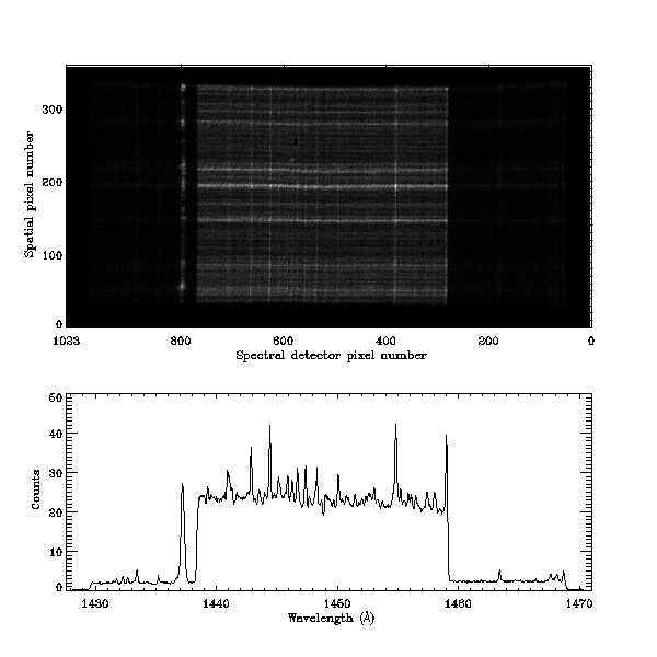
Figure
1.2:
1.2 SUMER
Reduction of
A step-by-step description
of the routines used for the reduction of
In the case of SUMER FITS
files a unique routine (calling all the necessary ones) has been written by K.
Bocchialini and P. Lemaire. Further information can be found at the MEDOC site.
1.2.1
Dead-time & local gain correction
For a total counting rate
greater than 5 x 10⁴ event s-1, a correction for the
electronic dead-time effect needs to be applied (Wilhelm et al. 1995; Hollandt
et al. 1996). It is important to bear in mind that, whether or not only a part
of the detector (sub-format image) is telemetered to the ground, the full
detector area has been exposed. Thus, the total count rate on the detector
cannot be inferred from the total counts in an image if sub-format images are
used. In the last case the XEVENT and YEVENT
parameters, that can be obtained from the header of the IDL-restore files (not
the FITS or FTS header), needs to be used. Alternatively, if the full spectral
image is also available (such an exposure is generally taken in the course of a
sequence), it is possible to evaluate the ratio between the counts in the area
corresponding to the sub-format image and the counts in the full detector
frame. In this case the full detector count rate for each sub-format image can
be estimated dividing the total counts in the sub-format image for the above
ratio.
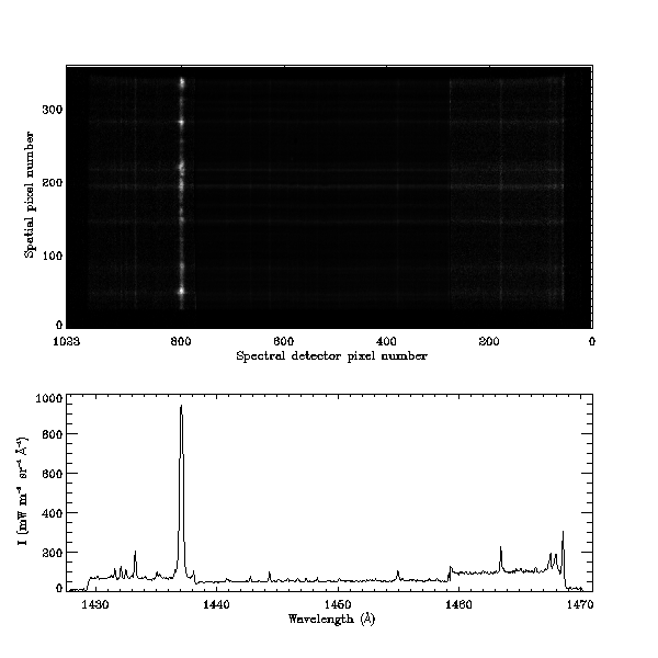
Another important effect
arises when, for certain bright lines (i.e. C III 977 Å or O VI 1032 Å), levels
around 10 counts pix-1 s-1 or higher are reached. In
these cases a local reduction in the micro-channel plate (MCP) gain and,
therefore, a loss of dynamic range will be present for such strong lines
(Wilhelm et al. 1997). In addition, long exposures of such bright lines at the
same pixel position on the detector will lead to a local reduction in the gain
after a certain amount of total counts (total charge) has been extracted. An
example of the last effect occurred after the full Sun scan in C III 977 Å on
28 January 1996 which left an imprint of reduced gain around detector (A) pixel
848 (see Fig.
1.2). In these
cases also a correction for the local gain depression needs to be applied at
the initial stage. Local gain correction requires dead-time correction to be
applied first.
Note that in cases of
particularly high local count-rates the line can produce a ghost around ~2.2 Å
towards higher wavelenghts (see section 2.2.4).
1.2.2
Flat-field correction
Flat-field correction is
necessary in order to correct for non-uniformities in the sensitivity of the
detector on scales of about 20 pixels or less. These are mostly due to a
non-linearity of the A/D-converters and the hexagonal pattern of microfiber
bundles of the MCPs. Flat-field images are taken approximatively every month
with a ~ 3 hour exposure in the Lyman continuum between 860 and 900 Å while the
spectrometer grating is de-focused (Schühle et al. 2000). In some cases the flat-field
correction is performed on board using the last acquired image. The flat-field
correction also eliminates or, at least greatly reduces, a modulation of
approximatively 19 % every two pixels in the spatial dimension caused by an
analogue-to-digital converter differential non-linearity (Siegmund et al.
1994). This gives us the possibility to verify whether an image was flat-field
corrected or not, simply by comparing a power spectrum of the averaged image
along the slit before and after the flat-field correction (Teriaca et al.
1999). The disappearance of the peak at period 2 is a clear signature that the
flat-field correction has been applied. However, in order to apply this
technique, it is important that the spectrum in question is characterized by a
sufficiently high signal-to-noise ratio. In Fig. 1.3 the Fourier analysis for the quiet Sun
spectrum shown in Fig. 1.2,
before and after the correction with a flat-field taken on 2 February 1996, is
presented.
Carlsson, Judge and Wilhelm
(1997) found a drift in the fixed pattern of the detector with time, which is
caused by scrubbing by the electrons extracted in the channel plates (Griffiths
et al. 1998). It is thus a function of the total charge extracted from the
channel plates. Since this depends on the location where bright spectral lines
have been registered on the active detector area, this is not uniform in time
and spatial location. It leads to a non-uniform drift of the fixed pattern,
except the 19 % pixel-to-pixel variation which is induced by the digitisation. It
is thus completely independent of the channel plate usage and is not moved by
this effect (Schühle, private communication). This drift can only roughly be
interpolated between subsequent flat-field exposures. In this way only a
temporal and spatial average of the drift can be determined. Since the 19 %
pixel-to-pixel variation, induced by the ADC, is a pattern that is not shifted,
it has to be corrected separatly, before a shifted flat-field correction is
applied. For this purpose, the SUMER calibration data base provides an image
(for A and B detector each) that can be applied to the data by using the
flat-field correction routine. This will remove the odd-even row pattern from
the data by multiplication of an ODD_EVEN_ARRAY. Of course, in
this case, flat-fields with the odd-even pattern removed must be used.
In general, when the data
and the closest flat-field are only few days apart, the drift should be small. Teriaca
et al. (1999) found a drift of 0.037 pixels (in the spectral direction) between
data and a flat-field ~3 days apart. This corresponds to approx. 0.4 km s-1
at 1250 Å. Such a drift is, however, much smaller then the residual errors in
the geometrical distortion correction (see below) and can be ignored. However,
attention must be paied when the data and the closest available flat-field are
many days apart.
In the case of some particular observations (e.g. large rasters of the quiet Sun) a technique to extract the flat-field matrix directly from the data has been described by Dammasch et al. (1999).
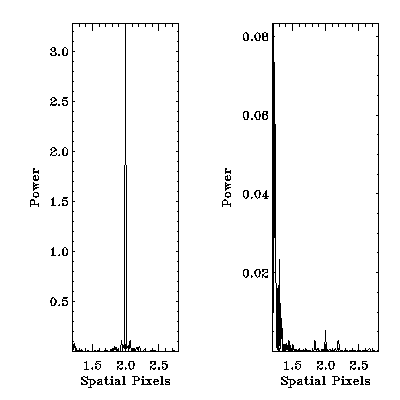
Figure
1.3: Power spectrum of the average along the slit of the Quiet Sun detector
image showed in Fig. 1.2, before (left) and
after (right) the flat-field correction, showing the reduction in the
electronic modulation (see Teriaca et al. 1999, for another example).
1.2.3
Geometrical distortion
The electronic design of
the detector induces a geometrical distortion of the images produced by
1.2.4
Radiometric calibration
The radiometric calibration
of the
In-flight calibration
curves were obtained through an iterative process leading to a continual
improvement in the final result. Calibration curves were first refined in
flight for both orders and for both photocathodes with the help of star data
and line ratio methods (Wilhelm et al. 1997). These results have been compared
with data from other UV instruments, and particularly from SOLSTICE (Woods et
al. 1998). After the comparison (Wilhelm et al. 1999), responsivity curves were
revised and are now available for the KBr photocathode and the bare MCP,
respectively (see Fig. 1.4). Uncertainties
for detector A are estimated to be 15 % from 540 to 1205 Å, 30 % above 1250 Å
on KBr. Below 540 Å only very few lines can be observed, and the data need
further confirmation. At this stage the uncertainty is estimated to 50 % (1
sigma) (Wilhelm et al. 2000). The KBr data for detector A in this range need
further study. In order to increase the life-time of detector B, in September
1996 it was decided to operate it at a lower gain than during the calibration
phase in laboratory. This led to larger uncertainties in the responsivity
curves. Uncertainty below 540 Å remains as high as 50 %. In the main part of
the spectral range, from 540 Å to 1236 Å, the uncertainty is below 20 %
(Schühle et al. 2000). The radiometric calibration is performed through the
provided software (RADIOMETRY.PRO, written by K. Wilhelm). Responsivity
curves are subjected to continuous study and can be changed from time to time. Hence,
it is very important to make sure that the latest calibration is used.
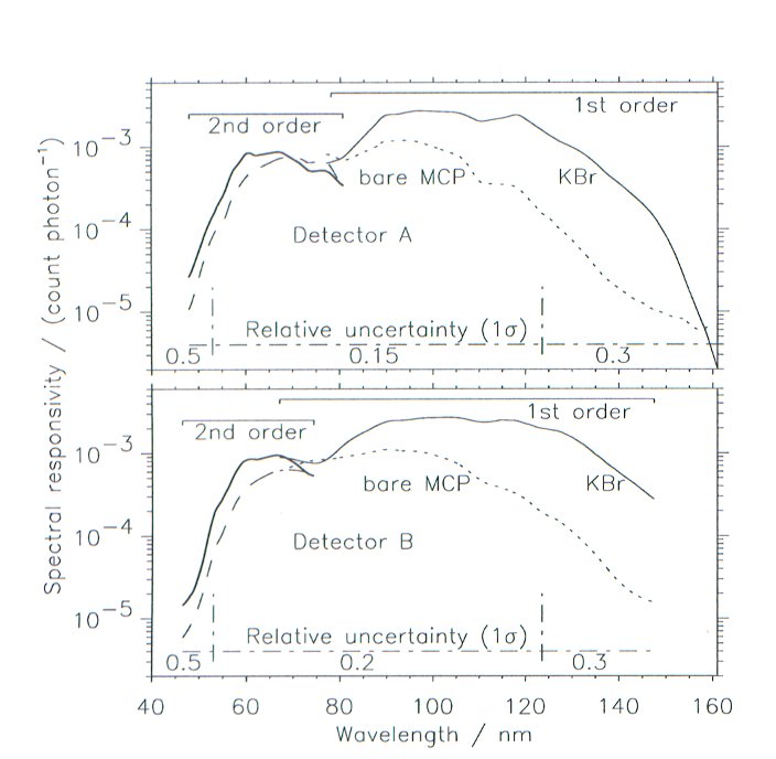
Figure
1.4: Spectral responsivity curves for
Figure
1.5:
1.2.5
Wavelength calibration
Particular attention needs
to be paid to the problem of the wavelength calibration. In the case of
Figure
1.6:
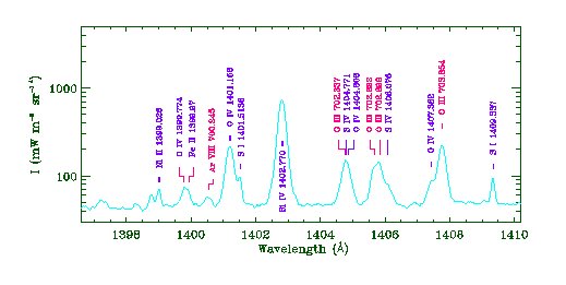
A careful measurement of
the absolute line position of several spectral lines across the
A preliminary wavelength scale was found for every spectrum using the information contained in the data header (wavelength of reference pixel). In fact, considering the grating equation, we have:
|
|
[1] |
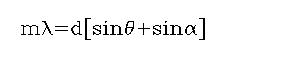
where m is the
diffraction order, d is the grating spacing, ![]() the angle of incidence on the grating and
the angle of incidence on the grating and ![]() the angle of reflection off the
grating. In the case of detector A, sin (
the angle of reflection off the
grating. In the case of detector A, sin (![]() ) =0 while for detector B we have:
) =0 while for detector B we have:
|
|
[2] |
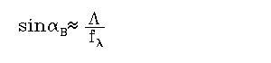
where ![]() is the distance between the centres of the two
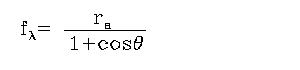
detectors. For a spherical concave grating of radius ra (= 3200.78
mm), the effective focal length is given by:
is the distance between the centres of the two
detectors. For a spherical concave grating of radius ra (= 3200.78
mm), the effective focal length is given by:
|
|
[3] |
Consider the case of
detector A, cos (![]() )=1. Differentiating
Eq.1 with
)=1. Differentiating
Eq.1 with ![]() kept
constant and assuming f
kept
constant and assuming f![]() /
d
/
d ![]() = dx (where dx
is the scale of the resolution, given by the pixel size in the spectral
direction), we obtain:
= dx (where dx
is the scale of the resolution, given by the pixel size in the spectral
direction), we obtain:
|
|
[4] |
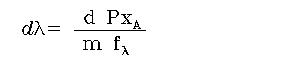
where PxA
is the spectral size of the pixels in detector A (26.6 µm, see Table 1.1). The dispersion value in the
header of FITS files results from the above equation. Combining Eq.1, Eq.3 and
Eq.4, we can write the dispersion as a function of the wavelength for detector
A,
|
|
[5] |
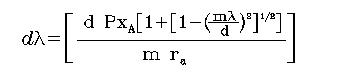
The above equation can be
used to build-up a preliminary dispersion relation, which is used as a starting
point for the identification of the chromospheric spectral lines present in the
spectra. Lists of lines observed on the Sun (on disk and off disk) are
available in the literature (Curdt et al. 1997a, 2001; Kink et al. 1997;
Feldman et al. 1997; Sandlin et al. 1986; Noyes et al. 1985; Cohen et al. 1978;
Vernazza & Reeves 1978; Behring et al. 1976). For laboratory wavelengths of
UV spectral lines, a large dataset can be found in the literature (Kelly 1982,
1985, 1987) and on the Internet (, e.g., Harvard-Smithsonian Center for Astrophysics
Databases and the National Institute of Standard and Technology on-line energy level database).
After having identified as
many chromospheric lines as possible, a Gaussian fit was applied to each one in
order to derive its central position (in pixels). For each region of interest
the dispersion relation was, hence, calculated performing a first order
polynomial fit to the pairs `central pixel'-`laboratory wavelength' of the
reference lines. This allows us to determine an absolute wavelength scale,
making it possible to measure the central wavelength of all the other spectral
lines. The use of a first order fit implies the assumption that the dispersion
relation is locally linear. This assumption can be defended observing that the
theoretical dispersion obtained from Eq.5 (see also Fig. 1.7) shows a small dependence on the wavelength,
so that it can be considered constant in intervals of ~20 Å. The derived
dispersion values are reported in Table 1.2. In Fig. 1.7 the dispersion values reported in Table 1.2 are shown together with the results
obtained by Chae et al. (1998a) and with the theoretical trend from Eq.5. It
can be noted how both the results from Teriaca et al. (1999) and Chae et al.
(1998a) are slightly lower than the values obtained through Eq.5. Generally the
laboratory wavelengths of chromospheric lines are well known, with errors much
smaller than 1 km s-1.
Table 1.2: Dispersion values for different spectral regions as measured
in the Quiet Sun and in Active Region NOAA 7946. Wavelengths for Iron lines are
taken from Kelly (1985), all the others from Kelly (1982). In the first column,
together with the spectral range, are also listed some of the ionic lines
present in that range.
|
Spectral Range
(Å) |
Ref. line |
Disp. (Å/pix) |
|
1560 - 1590 (AR) |
Fe II 1563.790 |
0.04166 |
|
Fe II 1569.674 |
||
|
Fe II 1570.244 |
||
|
Fe II 1571.137 |
||
|
Fe II 1581.270 |
||
|
Fe II 1584.952 |
||
|
Fe II 1588.290 |
||
|
1540 - 1570 (AR) |
Fe II 1550.274 |
0.04176 |
|
Fe II 1559.085 |
||
|
Fe II 1563.790 |
||
|
Fe II 1569.674 |
||
|
Fe II 1570.244 |
||
|
1520 - 1550 (QS) |
Si II 1526.7076 |
0.04180 |
|
Si II 1533.4320 |
||
|
C I 1542.1766 |
||
|
1380 - 1405 (AR) |
Fe II 1387.219 |
0.04257 |
|
Fe II 1392.149 |
||
|
S I 1392.5878 |
||
|
Fe II 1392.817 |
||
|
S I 1401.5136 |
||
|
1350 - 1365 (AR) |
C I 1354.288 |
0.04266 |
|
C I 1355.844 |
||
|
C I 1357.134 |
||
|
C I 1357.659 |
||
|
C I 1358.188 |
||
|
C I 1359.275 |
||
|
C I 1359.438 |
||
|
C I 1364.164 |
||
|
1295 - 1320 (AR) |
S I 1295.6526 |
0.04286 |
|
S I 1300.907 |
||
|
C I 1310.637 |
||
|
C I 1311.363 |
||
|
C I 1311.924 |
||
|
C I 1312.247 |
||
|
1250 - 1270 (AR) |
C I 1254.513 |
0.04296 |
|
Si I 1258.795 |
||
|
S I 1262.8596 |
||
|
S I 1270.7821 |
||
|
1240 - 1255 (AR) |
C I 1244.535 |
0.04307 |
|
C I 1245.943 |
||
|
C I 1249.004 |
||
|
C I 1249.405 |
||
|
C I 1252.208 |
||
|
C I 1254.513 |
||
|
1025 - 1045 (QS) |
O I 1027.4307 |
0.04391 |
|
O I 1028.1571 |
||
|
O I 1039.2304 |
||
|
O I 1040.9425 |
||
|
O I 1041.6876 |
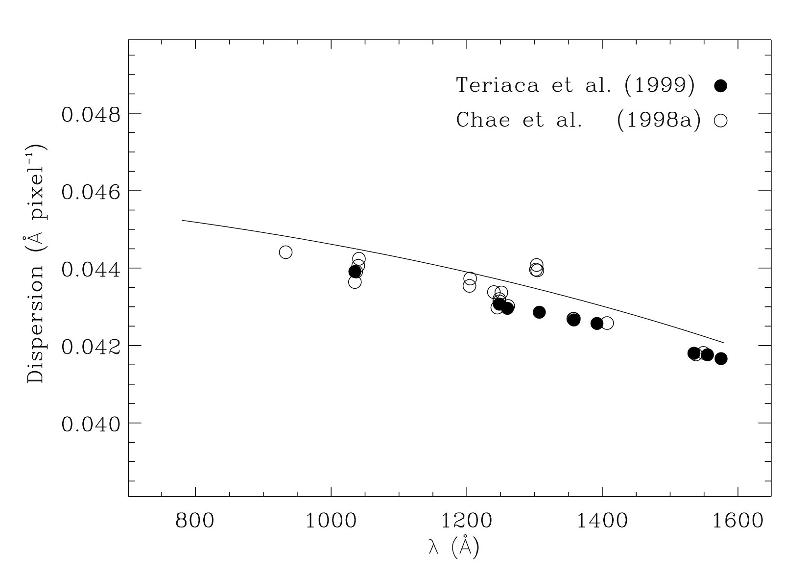
Figure
1.7: Spectral dispersion for detector A: theoretical and observational results.
The solid line represents the theoretical dispersion values for Detector A as
obtained through Eq.5. Dispersion values obtained using chromospheric lines are
also shown. Results represented by filled circles are from Teriaca et al. (1999),
while open circles indicate values obtained by Chae et al. (1998a).
1.2.6
Additional corrections
After having applied all
the above corrections, the spectra are ready to be analyzed. However, there are
some other corrections that are important to apply in particular cases.
1.2.6.1
Instrumental broadening
This is a problem common to
any spectroscopic analysis and concerns the fact that recorded line profiles
are the result of the convolution of the instrumental profile with the true
flux spectrum (Gray 1992). Emission lines arising from optically thin
transition region and coronal plasma can be considered Gaussian in shape to a
very good approximation (Mariska 1992). This is not strictly true for the
instrumental profile. This implies that, in theory, the recorded spectral
profiles should be not Gaussian in shape leading to the necessity of
deconvolution processes of the data in order to extract the ``true'' spectrum. This
is not a trivial operation with complications coming from the almost
unavoidable presence of noise, data sampling and windowing (Gray 1992). Moreover,
in order to perform the reconstruction process we should have the instrumental
profiles for all the possible detector-grating angle-slit combinations. These
profiles can be obtained in laboratory before the launch, but not during the
flight (there are no calibration lamps aboard). However, in the large majority
of cases (outside dynamic events and for lines formed in an optically thin
plasma),
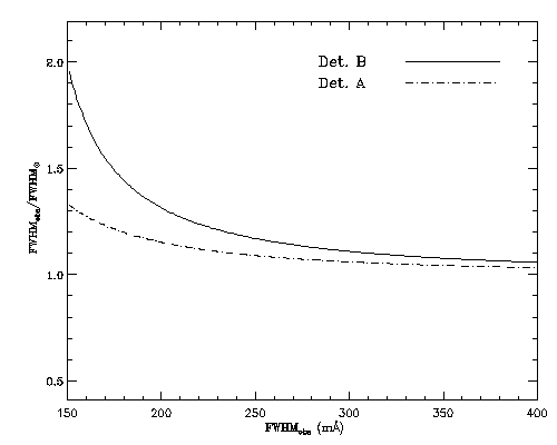
Figure
1.8: The ratio between the observed FWHM (FWHMobs) and the corrected
one (FWHMsun) is shown for both detectors as a function of FWHMobs.
1.2.6.2 Slit
magnification and displacement
The existence of a
discrepancy between the orientation of the grating and the detector, causes the
spectrum to be inclined with respect to the detector horizontal lines. This
leads to a change in the vertical position of the slit image on the detector
plane as a function of wavelength. Moreover, the position of the slit image on
the detector is also shifted due to the nonlinearity of the grating focus
mechanism which is moved simultaneously with the wavelength scan. And, last but
not least, there may be a residual angle between the scan mirror rotation axis
and the detector vertical lines, which may contribute to the displacement of
the slit image.
Besides the displacement of
the whole slit image, its projected size on the detector plane is also wavelength
dependent. The scale of the Sun image focused by the primary mirror on the slit
plane is 6.316 µm arcsec-1. This leads the long (1.89 mm) slit to
cover 299.2 arcsec while the short (0.755 mm) slit will cover 119.6 arcsec (see
Table
1.1). The slit is
then projected by the collimator over the grating, which will finally focus
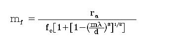
monochromatic images of the slit onto the detectors (see Fig. 1.1). The final size of the slit image on the
detector plane is determined by the ratio between the grating effective focal
length f![]() and the collimator focal length fc, the so-called magnification
factor. In the case of detector A (sin(
and the collimator focal length fc, the so-called magnification
factor. In the case of detector A (sin(![]() )=0), combining Eq.1 and Eq.5 we can easily
obtain the magnification factor mf as a function of wavelength,
)=0), combining Eq.1 and Eq.5 we can easily
obtain the magnification factor mf as a function of wavelength,
|
|
[6] |
Using the value obtained
from Eq.6, we finally obtain the spatial scale of the image on the plane of
detector A as:
|
|
[7] |
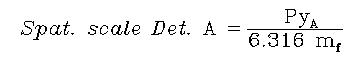
where PyA is the
spatial size of the detector pixels (26.5 µm, see Table 1.1). From the last equation it is easy
to calculate that the long slit will cover 291 and 315 spatial pixels of
detector A at 800 Å and 1600 Å respectively. In Fig. 1.9a, the spatial scale of the slit
image on the detector planes are shown as a function of the wavelength for both
detectors.
The combined effects of the
slit image displacement and magnification translate into the fact that, as an
example, a solar feature recorded on detector A spatial pixel 179 at 1238 Å (N
V) will be recorded around pixel 164 when observed at 1548 Å (C IV). The amount
of displacement can be as high as 21 spatial pixels, corresponding to ~ 15000
km on the Sun surface. In Fig. 1.9b the spatial position (in detector pixels) of a point
of the slit image falling on detector pixel 179 at 1238 Å, is shown as a
function of wavelength for both detectors. The above correction needs to be
applied only when comparing images obtained at different wavelengths. The
vertical displacement and spatial scale of the slit image as a function of
wavelength can be determined using the provided software (DELTA_PIXEL.PRO and MAGNIFICATION.PRO, respectively).
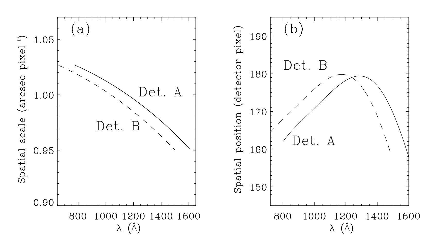
Figure
1.9: Slit image scale and spatial displacement on the detector planes as a
function of wavelength. (a): Image spatial scale as function of wavelength on
detectors A (solid line) and B (dashed line). (b): Spatial position (in
detector pixels) of a point of the slit image, falling on detector pixel 179 at
1238 Å, as a function of wavelength in the cases of detector A (solid line) and
B (dashed line).
1.2.6.3 Long-
and short-time instrumental periodicities
Despite the very high
thermal and mechanical stability characterizing the instrument (the temperature
inside the spectrometer compartment being controlled to within ± 0.15 K,
Wilhelm et al. 1997), a drift of the whole spectral image has been detected by
Curdt et al. (1997b). This periodic drift is due to thermoelastic oscillations.
It was later found also by Dammasch et al. (1999), Peter (1999a, 1999b),
Muglach & Fleck (1999) and Rybák et al. (1999a). In all these cases, the
authors report a periodic drift with an amplitude up to 1 pixel and a
periodicity of 1-2 hours. We interpreted these oscillations as the effect of
mechanical deformations of the spectrometer structure due to small temperature
changes induced by the spectrometer heaters. The drift can be avoided by
switching off the heaters during the observational sequence (W. Curdt, personal
communication). The problem appears whenever a sequence involves a considerable
amount of time. This is true in the case of temporal series (i.e. sequences of
spectra obtained keeping the slit fixed over the same point on the solar surface)
devoted to the study of solar chromospheric, transition region and coronal
oscillations as well as in raster scans (the slit is moved to an adjacent
position after each exposure) of large areas of the solar surface. The drift
can assessed looking at the behaviour of the mean line position averaged over
all the individual line positions along the slit. In fact, the average along
the slit greatly reduces the variations of solar origin, and the large scale
variations of the mean position through the dataset will underline the presence
of the instrumental drift. A spline fit, or a smoothing procedure, can be
applied to the mean line position in order to remove residual variations of
solar origin, obtaining a good estimation of the large-scale instrumental drift
(see Fig. 2 in Peter 1999a and discussion therein). The drift so obtained can
hence be subtracted. Of course, the determination of the drift is more accurate
when it can be obtained averaging the results of various lines.
A possible problem also exists
for temporal series during which a compensation for the solar rotation is
applied (Rybák et al. 1999b). These authors suggest that the stepping mechanism
could introduce spurious frequencies in the power spectrum of solar
oscillations. In the case of temporal series obtained without compensation for
the solar rotation there is no problem of introducing short-period variations,
but attention has to be paid to the fact that features drift across the strip
of solar surface imaged by the slit.
Luca Teriaca, teriaca@mps.mpg.de
Udo Schühle, schuehle@mps.mpg.de
Last update: 31.October.2014