 Observations and data analysis
Observations and data analysis
Observations and data analysis
The SoHO spacecraft and its 12 experiments allow us to observe the Sun from its central core up to the extended corona. In particular, the SUMER spectrograph is able to obtain spectra and monochromatic images of the solar chromosphere, transition region and low corona with high spatial, spectral and temporal resolution. The pointing mechanism of the instrument allows coverage of the entire solar disk and its surroundings up to 1 Rsun above the limb, permitting observational sequences devoted to the study of different regions of the solar atmosphere. In this Chapter a description of the principal data analysis techniques is presented.
As already mentioned, the SUMER spectrograph allows several different types of observational sequences, often complementing one another. In the spectral scan, the entire wavelength range is scanned, taking care to record each line with both the KBr and the bare part of the detector (in order to distinguish between first and second order lines). In the raster scan, a specific area of the Sun surface (but also of its corona) is scanned moving the slit in the direction perpendicular to the slit itself. Often, essentially because of constraints due to the telemetry rate and to the available memory on board, only selected spectral windows are telemetered to the ground. In the temporal serial, the slit is kept on a fixed location and successive spectra are taken at the same central wavelength. In the spatial spectrum a single, full detector spectrum, is obtained with high exposure time. This last type of observation is often prior to and after the raster scan and the temporal serial sequences in order to provide the full reference detector image from which the line(s) used in the temporal or raster sequences are extracted. In half detector, a subframe of 512 spectral pixels by 360 spatial pixel is telemetered to the ground.
After recording, the data can undergo a compression procedure, in order to reduce the transmission time (see Wilhelm et al. 1995 for more details). Images are, hence, telemetered to the ground together with a descriptional header, containing information about the performed observations (e.g. exposure time, central wavelength-reference pixel, slit and detector used, etc). These raw data are stored on CD--ROMs by NASA, and they are also stored as FITS (Flexible Image Transport System) files in the EOF (Experimenters' Operation Facility) at the Goddard Space Flight Center (GSFC) in Washington D.C. These FITS files contain an additional descriptive header, including information from the planning process. Starting from January 1996, the FITS files are currently reprocessed from the original CD--ROM data, with the purpose of improving the quality and removing data faults. The reprocessed data are saved with the extension .FTS (instead of .FITS). It is of fundamental importance to bear in mind that SUMER is fixed ``head-down'' on SoHO, hence the north direction on the Sun is towards the bottom of the detectors (i.e. images are upside-down). This has been changed in the reprocessed (.FTS) files where the north on the Sun is on the top of the image. Data can be found in both formats, and special care need to be paid to the problem when writing the reduction and analysis software.
Compensation of the solar rotation is achieved by moving the slit westward
of a given number of elementary steps. If the default rotational compensation
is chosen (ROTCOMP=0) then a double step (~0.76 arcsec) is performed every
 t seconds, where t
is a function of the pointing coordinates and the distance between SOHO and
the sub-SOHO point (see Wilhelm et al. 1995).
The rotational compensation can also be personalized by providing the time
interval after wich a double step is performed. Of course, the compensation
can also be performed by providing starting coordinates, for each spectroheliogram
of a series, that account for the interlapsed rotation.
t seconds, where t
is a function of the pointing coordinates and the distance between SOHO and
the sub-SOHO point (see Wilhelm et al. 1995).
The rotational compensation can also be personalized by providing the time
interval after wich a double step is performed. Of course, the compensation
can also be performed by providing starting coordinates, for each spectroheliogram
of a series, that account for the interlapsed rotation.
It is important to underline that the rotation compensation is NOT applied within a raster or a temporal series (defined as a spectroheliogram with spatial increment equal to zero) even if the rotation compensation was enabled during the study. As an example let us consider a study consisting of 2 rasters of a region around Sun center and that the standard rotation compensation is ON. Let also assume that the observed area is covered in 89 steps of 1.13 arcsec (3 elementary steps) each one followed by a 40 seconds exposure. This mean that each raster lasts one hour and covers formally a 100 arcsec wide region. However, because the rotation compensation is not active during each raster and the solar rotation is around 10 arcsec/hour at disk center, each raster will cover an area that is 10 arcsec wider or smaller, depending on whether the raster is achieved stepping eastward or westward. This is relevant when comparing a raster with an image (e.g., with a magnetogram). Moreover, because the rotation compensation is active during the study, the second raster will start at a pointing position 10 arcsec westward with respect to the starting position of the first raster. If a finer rotation compensation is required, this can be achieved by using several short rasters instead of a large one.
In the case of temporal series, the rotation compensation can be introduced using several small sequences, each one lasting the time after which the Sun has rotated of 0.76 arcsecs (see Section 1.2.6.3 for possible inconvinients).
The search for a compromise between the desire to obtain high (spatial, spectral and temporal) resolution observations and the need of a sufficiently high signal-to-noise to extract the requested information from the data, is a well known problem in astronomical observation in general and in spectroscopic analysis in particular. Thus, in some cases, the original data can be binned (in space and/or in time) in order to achieve a level of signal adequate to the specific analysis performed. The amount of binning, when necessary, needs to be carefully estimated in order to loose the minimum amount of information. Binning should be performed through a simple average of the reduced spectral profiles.
Brynildsen et al. (1998) have examined some SUMER and CDS images producing velocity maps (absolute for SUMER data and relative to the average velocity for CDS) in which they show an evident correlation between the observed redshift and the intensity of the line. Compared to the average wavelength position there is a tendency for the wavelength of the lines to change from blueshift to redshift as the peak intensity increases. Using SUMER observations in O VI and C II, Warren et al. (1997) found a slight dependence of line position and width on the intensity. Landi et al. (2000) divided a SUMER dataset in intensity bins and averaged all the profiles inside each bin, obtaining a high signal-to-noise spectrum for each intensity interval. A plot of the line parameters of these spectra against their intensity shows a clear dependence of both width and Doppler shift. There is, furthermore, evidence of a temporal, sometimes periodic, behaviour of the observed line shifts. This means that the (blue-) redshift phenomenon is of a statistical nature, with strong local variations in the observed Doppler shift in all the transition region lines. This last point is particularly important whenever we are interested in the measurement of the absolute amount of line shift presented by spectral lines. As discussed in Section 1.2.5 this is done using chromospheric lines to provide the wavelength calibration. However, these lines are usually quite weak and an average over several spatial positions is necessary in order to build-up a spectrum with a high signal-to-noise ratio. Also the short 120 arcsec slit is likely to cross more than one network region when used on the quiet Sun.
If a simple average (along the slit or over a whole image) is made, the locations with high redshift, being on average the most ``intense'', will dominate and the averaged value will be shifted towards more red shifted values. To avoid this, it is necessary to take some precautions. Chae et al. (1998a), solved the problem performing a weighted average along the slit, i.e. they normalize the line profile by the integrated intensity before an average is taken. Brynildsen et al. (1998), calculated the shift in every position along the slit and, afterwards performed the average along the slit. The last authors showed that the values obtained in this way are systematically lower that the ones obtained with a simple average, especially in active regions. It is also interesting to underline that they found practically no differential velocity between active and quiet regions, but this difference is present when they perform a simple average (with a maximum value around 5 km s-1 in O V). Teriaca et al. (1999) adopted the idea of Chae et al. (1998a) but they have also performed an average on the values calculated for every single spatial pixel for some spectra with very high signal-to-noise ratios. No relevant difference between the two methods was found.
The identification of the spectral lines present in a given spectrum is carried out through an extensive research in the literature (several works listing lines observed on- and off-disk are reported on Section 1.2.5, together with references to works reporting laboratory wavelengths). The identification of ionic lines can be helped by over-plotting the SUMER spectrum with a synthetic one, generated (for both orders) by the CHIANTI database (Dere et al. 1997; Landi et al. 1999). CHIANTI consists of a critically evaluated set of atomic data necessary to calculate the emission line spectrum of astrophysical plasma. It does not include transitions from neutral atoms. The data consist of atomic energy levels, atomic radiative data such as wavelengths, weighted oscillator strengths and A values, and electron collisional excitation rates. A set of programs that use these data to calculate the spectrum in a desired wavelength range as a function of temperature and density are also provided. These programs are written in Interactive Data Language (IDL), making it easy to couple them with the data reduction and analysis software. CHIANTI assumes an optically thin, low density static plasma in ionization and thermal equilibrium. In Fig. 2.1 and Fig. 2.2 two examples of SUMER spectra are shown (top) with superimposed the synthetic spectra (bottom) of first (dashes line) and second order (dotted line). The CHIANTI spectra were obtained using ionization equilibrium calculations from Mazzotta et al. (1998) and abundances values as measured by Grevesse & Sauval (1998) for quiet Sun and by Waljeski et al. (1994) for the active region spectrum.
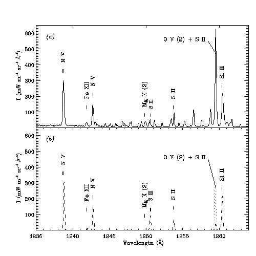
Figure 2.1: Comparison between SUMER quiet Sun spectrum (top) and CHIANTI synthetic spectrum (bottom) of first (dashed line) and second order (dotted line). Note the O V 629 Å and the Mg X 625 Å second order lines.
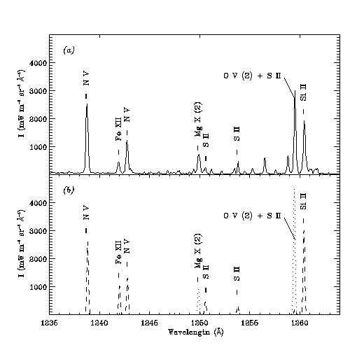
Figure 2.2: Comparison between SUMER active region spectrum (top) and CHIANTI synthetic spectrum (bottom) of first (dashed line) and second order (dotted line). Note the O V 629 Å and the Mg X 625 Å second order lines.
Despite the very high quality of the telescope mirror, the level of
scattered light is not negligible when observations of spectral lines which
are bright on disk (e.g. O VI, C II and L )
are carried out above
the limb in faint regions such as Polar Coronal Holes (Lemaire et al. 1997;
David et al. 1998). Here is reported as an example the analysis performed by
Banerjee et al. (2000) of a dataset obtained in June 1996 in the north polar
coronal hole plume and inter-plume regions.
An estimation of the stray light contribution to the O VI 1032 Å line
profile can be made using a purely chromospheric line such as C II 1037
Å (Hassler et al. 1997). This line does not have any coronal
contribution and is, hence, entirely due to stray light.
Fig. 2.3 shows the behaviour of the intensity with height
above the limb for O VI 1037 Å and C II 1037 Å lines.
Note the contrast between plume and inter-plume in O VI. If C II emission is
due only to scattered light we would not expect any difference between plume
and inter-plume (Hassler et al. 1997). The difference noted in
Fig. 2.3 near the disk is due to the
difficulty of fitting the C II line particularly when it is
only a tiny fraction of the nearby O VI 1037 Å line.
Furthermore a proper fit of the C II 1037 Å line was difficult
because the spectra nearest to the disk (up to ~ 1.2 solar radii were
only 50 pixel wide.
These problems lead essentially to an overestimation of the line width of
C II near the limb. In fact, it has been verified that the peak intensity
for C II shows the same values in plume and inter-plume. Data relative
to inter-plume were, hence, used for the calculation of the stray light
contribution.
The O VI 1032 stray light intensity at a certain altitude above the limb
will be given by the product of the C II 1037 intensity at that
altitude times the ratio of the disk-averaged O VI 1032 and C II
1037 line intensities.
The above ratio and the stray light profile in O VI 1032 Å
were evaluated using observations at 1.8 Rsun, where the
SUMER spectrum is entirely due to stray light (Lemaire et al. 1997).
)
are carried out above
the limb in faint regions such as Polar Coronal Holes (Lemaire et al. 1997;
David et al. 1998). Here is reported as an example the analysis performed by
Banerjee et al. (2000) of a dataset obtained in June 1996 in the north polar
coronal hole plume and inter-plume regions.
An estimation of the stray light contribution to the O VI 1032 Å line
profile can be made using a purely chromospheric line such as C II 1037
Å (Hassler et al. 1997). This line does not have any coronal
contribution and is, hence, entirely due to stray light.
Fig. 2.3 shows the behaviour of the intensity with height
above the limb for O VI 1037 Å and C II 1037 Å lines.
Note the contrast between plume and inter-plume in O VI. If C II emission is
due only to scattered light we would not expect any difference between plume
and inter-plume (Hassler et al. 1997). The difference noted in
Fig. 2.3 near the disk is due to the
difficulty of fitting the C II line particularly when it is
only a tiny fraction of the nearby O VI 1037 Å line.
Furthermore a proper fit of the C II 1037 Å line was difficult
because the spectra nearest to the disk (up to ~ 1.2 solar radii were
only 50 pixel wide.
These problems lead essentially to an overestimation of the line width of
C II near the limb. In fact, it has been verified that the peak intensity
for C II shows the same values in plume and inter-plume. Data relative
to inter-plume were, hence, used for the calculation of the stray light
contribution.
The O VI 1032 stray light intensity at a certain altitude above the limb
will be given by the product of the C II 1037 intensity at that
altitude times the ratio of the disk-averaged O VI 1032 and C II
1037 line intensities.
The above ratio and the stray light profile in O VI 1032 Å
were evaluated using observations at 1.8 Rsun, where the
SUMER spectrum is entirely due to stray light (Lemaire et al. 1997).
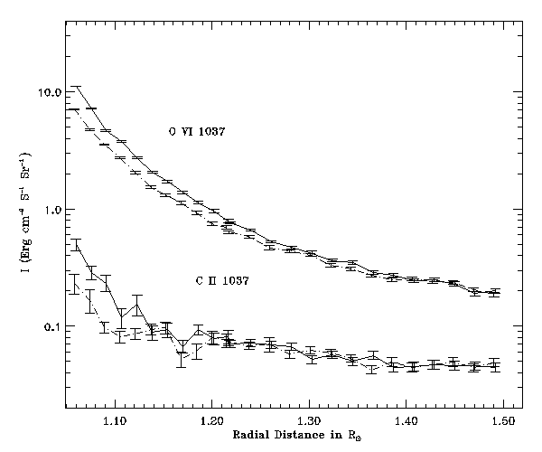
Figure 2.3: Variation of the intensity with height along a polar plume (solid line) and an inter-plume region (dashed l ine) for O VI 1037 Å and C II 1037 Å. From Banerjee et al. (2000).
Differences coming from the use of different detector and slit (in the case of the March 1997 observations) were taken into account in determining the width of the stray light profile. Assuming that the width of the O VI 1032 Å stray light profile does not vary with the height above the limb, its amplitude variation can be inferred from the stray light trend derived above. This allows the authors to obtain the stray light profile as a function of height and, finally, to remove it from the observed O VI profile. In Fig. 2.4 it is shown the variation of the O VI 1032 Å line intensity with height in the north polar coronal hole along a polar plume (dot-dashed line) and an inter-plume region (solid line). The dotted line represents the stray light contribution to the O VI line intensity. It clearly shows that, above 1.4 solar radii, the O VI intensity is entirely due to stray light.
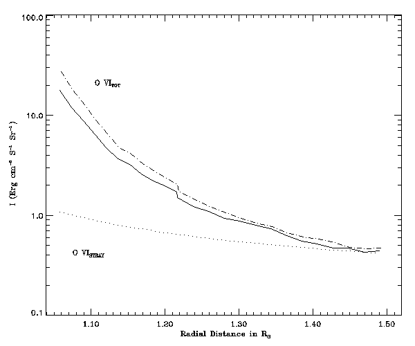
Figure 2.4: Variation of the O VI 1032 Å line intensity with height in the north polar coronal hole along a polar plume (dot-dashed line) and inter plume regions (solid line). The dotted line represents the stray light contribution to the O VI line intensity (adapted from Banerjee et al. 2000).
 ) heavily exceede the detector
capabilities. Then, in addition to dead-time losses, some pulses are
registered at a displaced position (~2.2 Å on the red side of the line)
and appear in both dimensions as ghosts in an image. Ghosts appear
particularly evident in off-limb observations of bright transients due to
the reduced continuum. Fig. 2.5 shows a clear example of
the spatial and the spectral ghosts produced by a very bright patch of
H I Ly emission (around pixels 770, 310).
Also the combined spectral and spatial ghost is clearly visible around
pixels 720, 260. In these cases great caution need to be paid to the values
obtained analysing the lines producing the ghosts. While the line intensity
is surely affected, it is not clear whether the line width and shift are
also affected and further study needs to be carried out.
) heavily exceede the detector
capabilities. Then, in addition to dead-time losses, some pulses are
registered at a displaced position (~2.2 Å on the red side of the line)
and appear in both dimensions as ghosts in an image. Ghosts appear
particularly evident in off-limb observations of bright transients due to
the reduced continuum. Fig. 2.5 shows a clear example of
the spatial and the spectral ghosts produced by a very bright patch of
H I Ly emission (around pixels 770, 310).
Also the combined spectral and spatial ghost is clearly visible around
pixels 720, 260. In these cases great caution need to be paid to the values
obtained analysing the lines producing the ghosts. While the line intensity
is surely affected, it is not clear whether the line width and shift are
also affected and further study needs to be carried out.
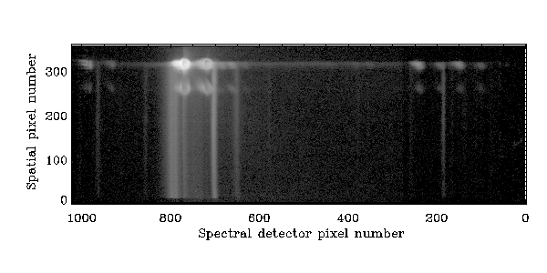
Figure 2.5: Logaritmically scaled image of the off-limb
corona during a transient event. Spectral range from 1208 to 1248
Å. A clear example of the spatial and the spectral ghosts produced
by a very bright patch of H I Ly emission
(around pixels 770, 310) is shown.
Also the combined spectral and spatial ghost is clearly visible around
pixels 720, 260.