|
|
|
|
Penumbral Structure |
(M. Rempel, M. Schüssler, R. Cameron, M. Knölker )
|
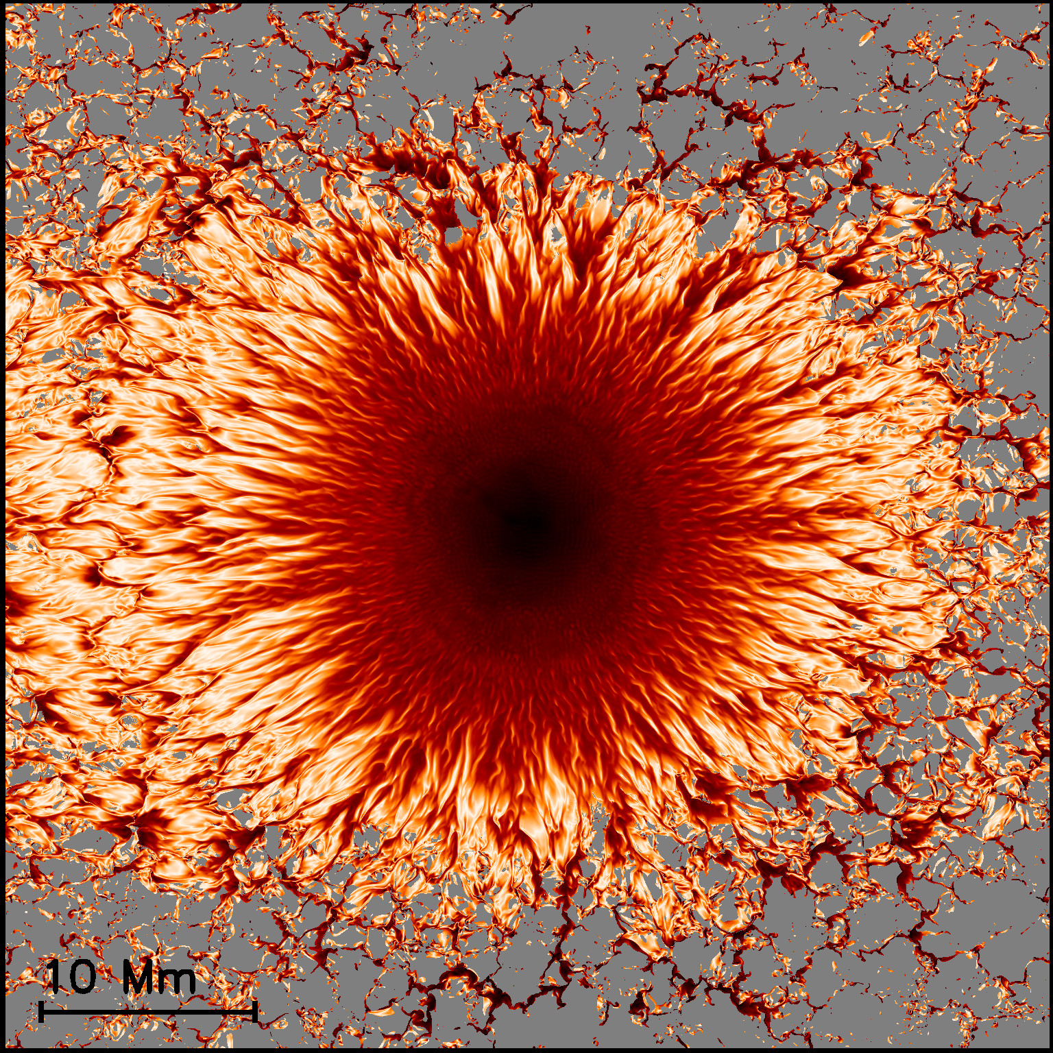
Figure 1: Inclination angle of magnetic field in and around a (simulated) sunspot (black is vertical field, white is horizontal).
|
The structure of sunspots, including their umbra, penumbra and the surrounding quiet-Sun has been simulated. The
simulations reveal the convective nature of the penumbra. The presence of the inclined magnetic fields in the penumbra
causes the convective motions to be highly anistopic, in terms of intensity (penumbral filaments with dark-cores,
outflows of up to 10km/s (the Evershed flow), and magnetic fields.
References
Penumbral Structure and Outflows in Simulated Sunspot
, Rempel, M., Schüssler, M., Cameron, R., Knölker, M., Science, Volume 325, 171-174 (2009).
Radiative Magnetohydrodynamic Simulation of Sunspot Structure
, Rempel, M., Schüssler, M., Knölker, M., ApJ, Volume 691, 640-649 (2009).
-> back to top |
|
|
Turbulent magnetic fields |
(J. Pietarila Graham, S. Danilovic, M. Schüssler )
Observations of small-scale magnetic fields fields from Hinode and
numerical simulations of dynamo action in the photospheric layers of
the Sun are compared. Using turbulence theory to motivate self-similar
scaling laws, a lower bound of 50G is derived for the unsigned quiet-Sun
vertical flux. This agrees with our MURaM simulation-based estimate
and (considering vector magnitudes) resolves the discrepancy between
Hanle and Zeeman observations.
|
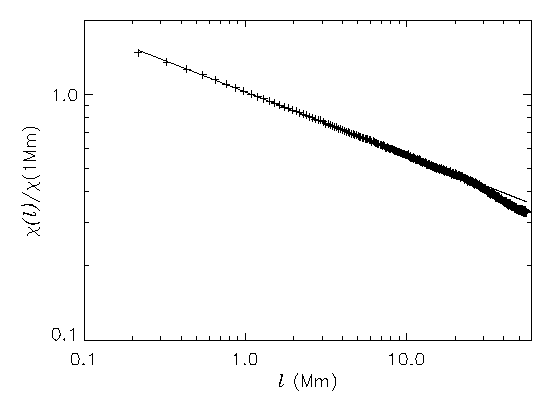
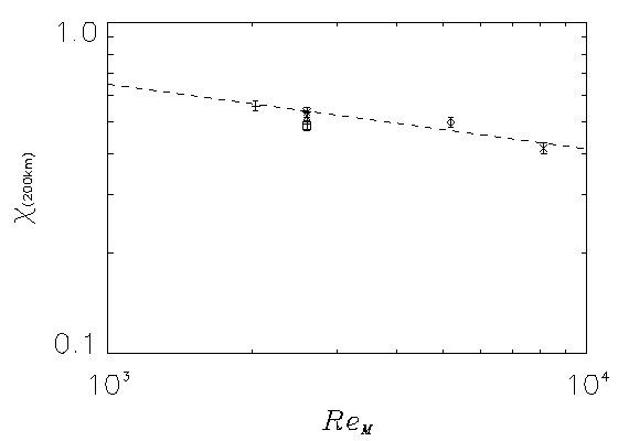
Figure 1. Left: Portion of magnetic flux remaining after averaging
over boxes of increasing size (from Hinode observation). A self-similar
power-law is abundantly clear for 2 decades of length scales down to the
resolution limit. Right: Flux remaining after averaging over
200 km X 200 km boxes for MURaM as a function of magnetic Reynolds
number, ReM. Extrapolation to solar ReM indicates at least 80%
cancellation at 200 km resolution.
|
|
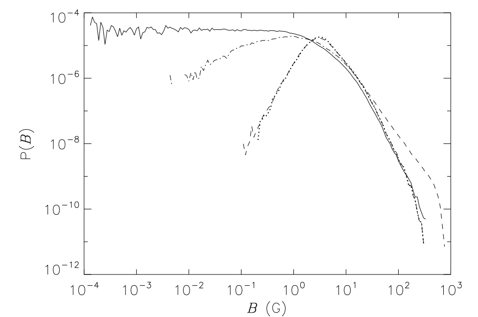
Figure 2. Probability distribution functions of magnetic field strengths
from the simulations (solid line), from the Hinode observations
(dashed lines), the inversions of synthetic stokes-diagnostics
created from the simulations (dash dot) and when an observational
noise level of 0.0011 is added (dotted line). The observational
peak that was previously considered solar is seen to be solely
due to noise.
|
References
Turbulent Magnetic Fields in the Quiet Sun: Implications of Hinode Observations and Small-Scale Dynamo
Simulations, Pietarila Graham, J., Danilovic, S., Schüssler, M., ApJ, Volume 693, 1728-1735 (2009).
-> back to top |
|
|
Identification of MURaM dynamo as a turbulent small-scale dynamo |
(J. Pietarila Graham, R. Cameron, M. Schüssler )
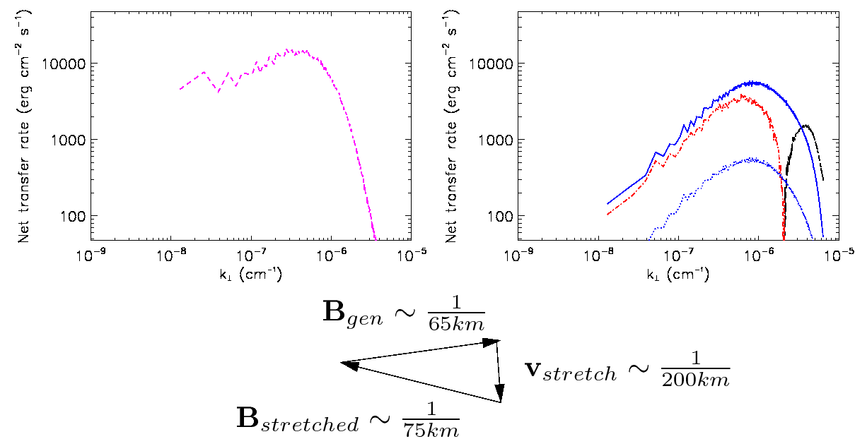
Spectral transfer analysis of the MURaM dynamo rules out the tangling
of magnetic field lines (turbulent cascade) and Alfvénization
of turbulent velocity fluctuations ("turbulent induction") as sources
of small-scale magnetic field (see Figure 1). Rather, small-scale
fluid motions stretch small-scale magnetic field to produce more
small-scale magnetic field and the scales involved become smaller with
increasing Reynolds number. This is a small-scale turbulent dynamo.
|
Figure 1. Transfer analysis of MURaM surface dynamo. Left: Work
against Lorentz force versus horizontal spatial frequency shows that
fluid motions at scales near 200 km stretch magnetic
field lines (dynamo). Right: Rate of magnetic energy production by
stretching (blue solid) and compression (blue dotted), magnetic energy
lost (red) and gained (black) from the turbulent cascade versus
horizontal spatial frequency. Magnetic field is produced predominantly
at scales near 65 km from stretching motions. Bottom: Triadic transfer
indicates the magnetic field that is stretched has scales near 75 km.
All scales are well below the 1000 km granulation scale, identifying
the dynamo mechanism as a turbulent small-scale dynamo.
|
|
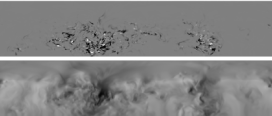
Figure 2. Vertical cuts of Top: Real-space analog of blue solid line
from Figure 1: rate of magnetic energy production by stretching and
Bottom: vertical velocity (dark for down-flows). Down-flow plumes are
the site of dynamo generation.
|
-> back to top |
|
|
Magnetoconvection in a sunspot umbra |
( M. Schüssler, A. Vögler)

|
Figure 1: Left frame: brightness;
Middle: vertical velocity (blue: upflows, red: downflows, white: stagnant
Right column: vertical magnetic field at <τ> = 1.
|
The strong magnetic field (from 2000 G to more than 4000 G) in a sunspot
umbra suppresses the normal granular convection. Simulations with the
MURaM code have shown that the convective energy transport instead
occurs in the form of narrow hot upflow plumes, which appear as bright
patches before a dark background (see brightness image to the left,
spatial scale in Mm). Their sizes, contrasts and lifetimes are similar
to the observed properties of so-called `umbral dots'.
The vertical velocity image (middle panel) taken near the level of
optical depth unity shows that the upflows in the plumes (blue) are
surrounded by narrow downflow channels (red). The strong expansion of
the upflow plumes with height due to the pressure stratification leads
to a strong expansion of the plumes and a concomitant reduction of the
magnetic field strength (right panel) in the upper layers. Near optical
depth unity, the hot material in the plume loses its buoyancy and piles
up in a cusp-shaped structure, leading to the appearance of dark lanes
in the brightness image.
Reference
Magnetoconvection in a Sunspot
Umbra, Schüssler, M. & Vögler, V., ApJ, Volume 641, Issue 1, pp. L73-L76 (2006).
-> back to top |
|
|
A solar surface dynamo |
( A. Vögler, M. Schüssler)
|
Figure 1: Left frame: brightness;
Middle: vertical velocity (blue: upflows, red: downflows, white: stagnant
Right column: vertical magnetic field at <τ> = 1.
|
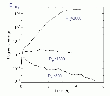
Various observations indicate the existence of significant amounts of
magnetic flux ubiquitous in the `quiet Sun', i.e., outside active
regions, with mixed polarity on small scales. Since idealized Boussinesq
closed-box simulations of Cattaneo (ApJ, 1999) showed dynamo action of
non-helical instationary convection, the existence of a similar process
based upon granular convection of the Sun has been discussed. Removing
the idealizations in a realistic simulation with the MURaM code, we have
found that solar surface convection seems indeed capable of supporting a
dynamo process: for sufficiently large magnetic Reynolds number, the
magnetic energy of an initial weak seed field grows exponentially and
saturates at levels consistent with the observational inferences. The
generated surface field has a small/scale structure with mixed polarity
(right panel: vertical field image near optical unity; the size of the
magnified inset is about 1200 km x 1200 km on the Sun) and shows an
association with the intergranular downflow lanes.
Reference
A solar surface dynamo, Vögler, A.; Schüssler, M., Astron. Astrophys., 465, L43-L46 (2007).
-> back to top |
|
|
Current sheets in the upper photosphere |
( M. Schüssler, R.Cameron, A. Vögler)
|
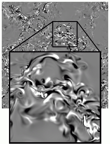
Figure 1: Left: vertical magnetic field at 600km above <τ> = 1
middle: Temperature;
Right: vertical velocity (blue: upflows, red: downflows, white: stagnant.
|
Simulations of mixed-polarity magnetic fields with the MURaM code reveal
the appearance of current sheets between field patches of opposite
polarity in the upper photosphere. The image shows a small section from
the highest-resolution and biggest simulation of solar
magneto-convection carried out so far: 5 km horizontal numerical cell
size and 1152 x 1152 x 200 cells. The image shows horizontal cuts of a
small part of the computational box at about 600 km above optical depth
unity (visible surface). The vertical magnetic field (left, black/white
color scale for the two polarities) shows a sharp polarity inversion,
which is outlined by a hot region in the temperature image (middle) and
associated with a strong downflow exceeding 10 km/s in the vertical
velocity image (right). The structure displays all characteristic
features of a `textbook' current sheet with reconnection: a
quasi-discontinuity of the magnetic field, local Joule heating and
temperature peak (exceeding 9000 K), horizontal inflow and vertical
outflow, local maxima of gas pressure and density. Possible
observational signatures are currently evaluated.
-> back to top |
|
|
Magneto-convection in the solar photosphere: From Quiet Sun
to strong plage |
(A. Vögler, M. Schüssler)
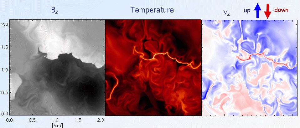
Using MURaM, we carried out a series of simulation runs to study
the dependence of photospheric magneto-convection on the amount
of magnetic flux. In each of the runs an initially vertical,
homogeneous magnetic field of strength B0 was introduced
into fully developed hydrodynamic convection.
We considered five cases with B0 = 10 G, 50 G, 200 G, 400 G, and 800 G.
Fig. 1 shows snapshots of brightness, magnetic field strength at<τ> = 1,
and vertical verlocity at<τ> = 1.
|
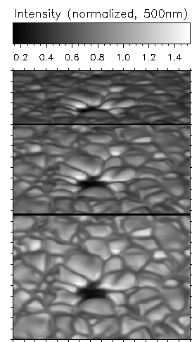
Figure 1: Snapshots for the cases with an initial field strength of
10 G, 50 G, 200 G, 400 G, and 800 G (from top to bottom).
Left column: vertical magnetic field at <τ> = 1; Middle column: brightness;
Right column: vertical velocity (blue: upflows, red: downflows, white: stagnant).
|
As a result of flux expulsion and convective field amplification, most of the
magnetic flux forms partially evacuated kilogauss flux concentrations embedded
in the network of intergranular downflows. In the case B0=10 G these field
concentrations are isolated flux tubes. With increasing flux, the strong
fields form a network on a mesoscale, with thin sheets in the downflow lanes
(see Fig. 2) and micropores at the vertices where several lanes merge.
As B0 grows, the granular pattern gets more and more disturbed and
the typical horizontal scales of granulation decrease.
|
Figure 2: 3D views of a thin magnetic sheet from two different angles. The shaded
surface in the upper panel is the isosurface τRoss = 1. The lower
panel shows a face-on view. The sheet loses its coherence in the
subsurface layers as the field lines get distorted by vigorous convective
flows.
|
|
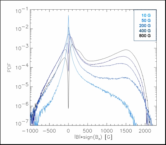
Figure 3: Probability density functions (PDF) of the magnetic field strength
around <τ> = 1. The distribution of the weak fields is a (stretched)
exponential. The strong field wing grows with increasing B0 and
is Gaussian. In the 10 G run, the maximum field strength around <τ> = 1
is significantly reduced. This finding is independent
of grid resolution and shows that the efficiency of convective
field amplification is reduced for small, optically thin flux concentrations.
|
Reference
- Simulations of magneto-convection in the solar photosphere: Equations, methods, and results of the MURaM code, A. Vögler, S. Shelyag, M. Schüssler, F. Cattaneo, T. Emonet, T. Linde, Astron. & Astrophys., in press.
- Simulating radiative magneto-convection in the solar photosphere, A. Vögler, in R. E. Schielicke (ed.): "The Sun and Planetary Systems - Paradigms for the Universe", Reviews in Modern Astronomy, no. 17, 2004.
-> back to top |
|
|
Decay of bipolar fields in the solar surface layers |
(A. Vögler, R. Cameron, M. Schüssler)
In a complementary line of simulations we studied the
structure and evolution of bipolar magnetic fields
in the photosphere and uppermost layers of the convection zone.
|
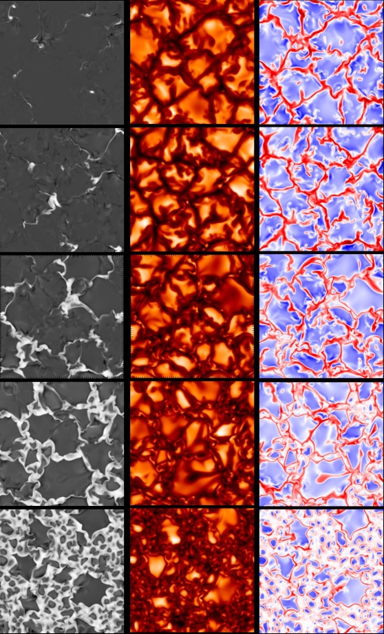
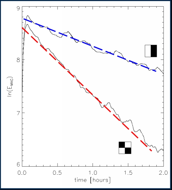
Figure 1: Exponential decay of the magnetic energy for two
mixed-polarity runs with different initial configurations
of the bipolar magnetic field ("checkerboard" and "striped").
The decay rates are consistent with the assumption of an effective
"turbulent" diffusivity ηt = 1.5 x 1012 cm2/s acting on the
fundamental Fourier modes of the respective field configurations.
|
|
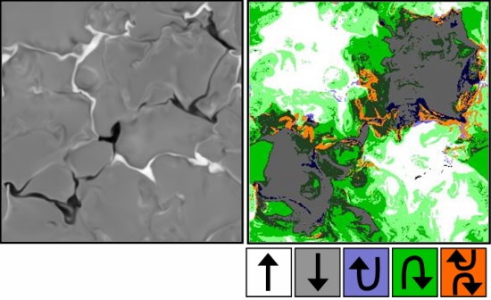
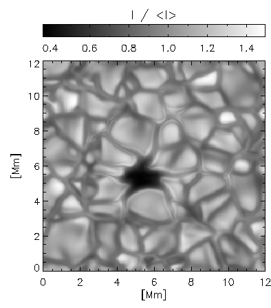
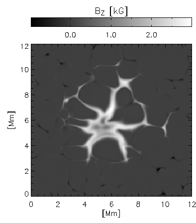
Figure 2: Left panel - Greyscale magnetogram of the "checkerboard" run at <τ> = 1, 20
minutes after the start of the simulation. The initial configuration
is still clearly visible. Right panel - Classification of the magnetic
field in four different topology classes: "up", "down", "U-loop", and
"inverse U-loop". Flux cancellation requires transformation of the
initial "up" and "down" flux into "U-loop" and "inverse U-loop" flux by reconnection. We find that most of the reconnection occurs in the upper photosphere where strong flux concentrations
of opposite polarity occasionally get into contact as they move in the
intergranular downflow-network in a random-walk style.
Accordingly, most of the "reconnected" flux around <τ> = 1 and below
occurs in form of inverse U-loops (green in Fig. 2, right panel).
Significant amounts of U-loop flux (blue) are only found in the
upper photosphere
|
|
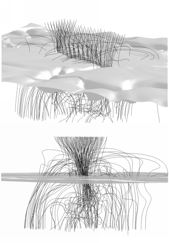
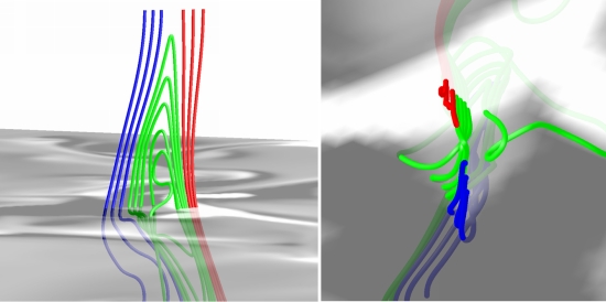
Figure 3: Field line plot of a reconnection event in the upper photosphere.
Left panel: side view; Right panel: top view. The translucent
plane shows the vertical field strength at <τ> = 1.
|
|
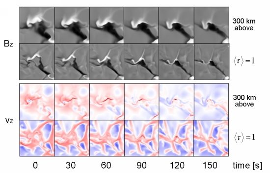
Fig.4: Time series of a flux-cancellation event. Upper two rows:
Vertical magnetic field at <τ> = 1 and 300 km above (strong fields
of either polarity are white and black, respectively).
Lower two rows: Vertical velocity (blue: upflow, red: downflow).
Each panel has a horiztonal extent of 2 x 2 Mm.
Owing to the expansion with height, strong field concentrations
of opposite polarity first touch in the upper photosphere when
moved into each other by convective flows. The time series
shows a clear downflow signature 300 km above <τ> = 1
at the current sheet separating
the two polarities. The downflow is triggered by the magnetic
tension force of inverse U-loops retracting into the underneath
layers. A weaker downflow signature is observed at <τ> = 1
with a time lag of about one minute.
|
-> back to top |
|
|
Simulation of solar pores |
(R. Cameron, A. Vögler, M. Schüssler)
 |  |
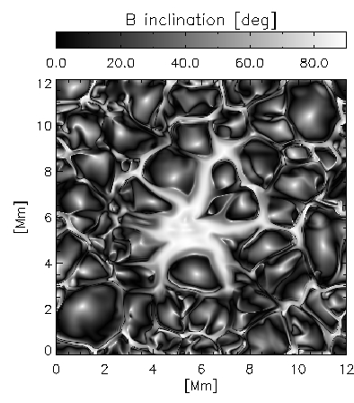 |
Figure 1: Pore properties at <τ> = 1. The top left panel shows a continuum brightness image, the panel above shows the vertical field strength and the left panel shows the magnetic field inclination. |
We have used the MURaM code to simulate a solar pore, in order to look at
its structure and evolution. Since the model incorporates realistic physics
for the photospheric layers, our simulations reproduce both qualitatively
(Figure 1) and quantitatively (Figure 2) the properties of pores. This
ability to reproduce the observations extends to observations away from
disk centre (Figure 3).
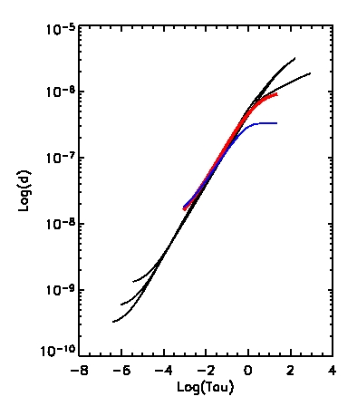 |  |
| Figure 2a: Height dependence of density as a function of optical depth in the pore. The three black curves are
from Sütterlin (observations), the red curve is from
a snapshot of our simulated pore, and the blue curve is our simulated quiet sun. |
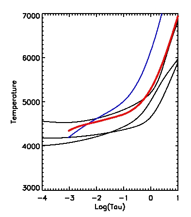
Figure 2b: Height dependence of temperature as a function of optical depth in the pore. The three black curves are
from Sütterlin (observations), the red curve is from
a snapshot of our simulated pore, and the blue curve is our simulated quiet sun. |
 |
| Figure 3: A side glance at the pore. |
Having reproduced the observations, we are then in a position to do what
is observationally impossible - look beneath the surface of the Sun and
directly at the magnetic field lines (Figure 4). In this way we can
understand how the physics which determine the form of the pore.
 |
 |
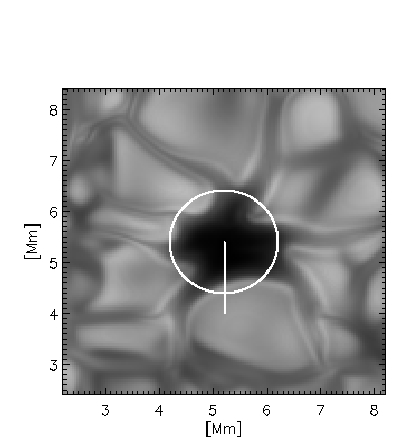 |
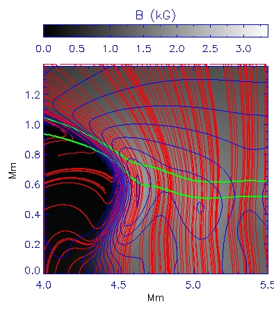
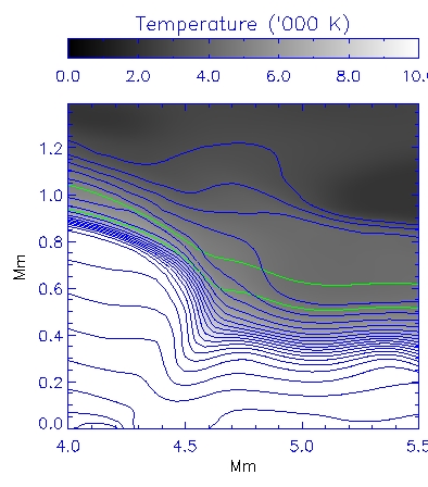
Figure 4: Shown in the upper left are the magnetic field strength (grey scale and
blue contours), the <τ>=1 and 0.1 surfaces (green lines), and the
direction of the magnetic field in the plane (blue streaks). The upper right panel
shows the temperature structure, whilst the left
panel shows the position of this slice.
|
Reference
Radiative magnetohydrodynamic simulations of solar pores,
Cameron, R., Schüssler, M., Vögler, A., Zakharov, V., Astron. Astrophys., in press
The decay of a simulated pore, R. Cameron, A. Vögler, S. Shelyag, M. Schüssler, in ASP Conference Series, Vol. 325, 2004.
-> back to top |
|
|
Magnetic flux emergence |
(M. Cheung, M. Schüssler)
|
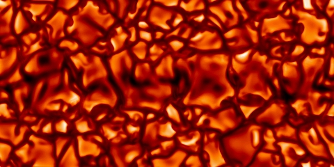
Figure 1: The footprint of emerging flux - Shown here is a brightness image of the photosphere from a simulation of an emerging flux tube. The emergence event is marked by the transient appearance of an elongated dark lane.
|
Magnetic flux emergence on the solar surface takes place over a wide range of fluxes and spatial scales. Studies of the emergence properties of bipolar active regions (Φ ∼ 1022 - 1023 Mx) and ephemeral regions (Φ = (3 - 300)×1018 Mx) indicate that magnetic flux at the larger length scales (10 - 102 Mm) emerge as coherent bundles of magnetic flux, commonly referred to as magnetic flux tubes.
We study the emergence process by means of numerical MHD simulations. For a proper treatment of the problem, it is important that the simulation code captures the essential physical ingredients in the photosphere, namely radiative transfer, partial ionization, and compressibility. The MURaM code satisfies all these requirements, and allows us to directly compare our simulation results with real photospheric observations of flux emergence. For example, Figure 1 shows a brightness image of a region of the photosphere (simulated) where a flux tube has just emerged. The site of emergence is marked by an elongated dark lane.
Magnetic flux emergence in granular convection: radiative MHD simulations and observational signatures, Cheung, M. C. M.; Schüssler, M.; Moreno-Insertis, F., Astron. Astrophys., 467, 703-719 (2007).
-> back to top |
|
|
|
Non-grey radiative transfer in radiative MHD simulations |
(A. Vögler, M. Schüssler)
Radiative transfer in realistic photospheric MHD simulations
needs to take into account the effect of line opacities in the
middle and upper photosphere. Owing to the sheer number of
lines, the modelling of these non-grey effects is statistical
in nature.
Non-grey radiative transfer in the MURaM code makes use of
the opacity binning concept which divides the opacity spectrum
into a handful (typically 4-5) of classes (bins) according to the
opacity strength ("strong lines", "weak lines", "continuum", etc.)
Based on a 1D reference atmosphere, the frequencies are classified
according to the geometrical height where<τ>ν = 1 is reached (Fig. 1). This
way each bin contains frequencies whose main contribution to the radiative
heating rate lies in the same height range.
 |
| Figure 1: The assignment of frequencies to bins is based on the (frequency-dependent) optical
depth scale τν. Frequencies, for which
τν = 1 is reached in the same range of geometrical
depth z, are assigned to the same bin. The solid line marks the geometrical depth
at τν = 1 as a function of frequency. |
Test calculations in a static 2D flux-sheet model show that
opacity binning does a rather good job of approximating the
reference solution obtained with high frequency resolution.
It turns out that the advantage over the grey appoach is particularly
pronounced in situations where inhomogeneities of the atmosphere lead to
lateral heating and cooling effects (Fig. 2). Owing to the inadequate
representation of line opacities, the grey radiative transfer is unable
to capture these effects and results in qualitatively wrong
radiative heating rates. Thus, non-grey radiative transfer modelling
is particularly important in MHD simulations which include strong magnetic
flux concentrations, because the partial evacuation of these fields leads
exactly to the kind of lateral inhomogeneities where the grey approach fails.
|  |
| Figure 2a: Reference solution of Qrad in a magnetic
flux-sheet model, obtained with high frequency resolution.
| Figure 2b: Horizontal cut at a height of z=300 km. The shaded region
marks the interior of the flux-sheet. While the opacity binning models perform rather well,
grey radiative transfer leads to qualitatively wrong heating rates.
|
Consequently, MURaM magneto-convection simulations carried out with
a four-bin non-grey radiative transfer significantly
differ from grey simulations in the height range τ ≤ 1:
- The average non-grey temperature profile differs from the grey profile in the
optically thin part of the computational domain. It shows the backwarming and
line cooling effects that are a familiar property of static 1D radiative
equilibrium atmospheres.
- The non-grey radiative transfer enhances the effect of radiative illumination
in magnetic flux concentrations (See Fig. 3).
|
| | Figure 3: Solid lines show the vertical temperature profiles inside magnetic structures with
above-average brightness. Dashed lines show the mean temperature profiles of the whole
simulated domain. Red lines correspond to the non-grey, black ones to the grey
simulation run. |
- The use of a non-grey radiative transfer leads to a significant decrease of
temperature fluctuations in the upper photosphere (Fig. 4). In the grey case,
the Rosseland mean underestimates the strength of absorbers and does not allow
an adequate modelling of the smoothing effects of the radiative transfer. The
difference is particularly pronounced in magnetic field concentrations.
| Figure 4: Vertical profiles of the horizontally averaged temperature fluctuations inside
strong magnetic flux concentrations. The non-grey radiative energy exchange strongly reduces
temperature fluctuations in the upper photosphere. |
- The differences in the temperature structure affect the appearance of the
simulations in brightness maps: the rms intensity contrast is reduced to 15%
in the non-grey case compared with 18% in the grey case. This reduction of
the overall contrast leads to a contrast enhancement of bright magnetic elements
(Fig. 5).
| Figure 5: Maps of frequency-integrated intensity for the grey ( left panel) and non-grey (
right panel) simulation runs, using the same color coding for both images. In
the non-grey case, granules are darker and the overall contrast is reduced. As a
result, bright magnetic features stand out more prominently. |
Reference
- Effects of non-grey radiative transfer on 3D simulations of solar magneto-convection, A. Vögler, Astron. & Astrophys., 421, 755-762, 2004.
- Approximations for non-grey radiative transfer in numerical simulations of the solar photosphere, A. Vögler, J. H. M. J. Bruls, and M. Schüssler, Astron. & Astrophys., 421, 741-754, 2004.
-> back to top |
|
|
|
|
|
|
|
|
|
Contact: Robert Cameron
|
|