Research Projects

Revealing migration properties of the Sun's magnetic field
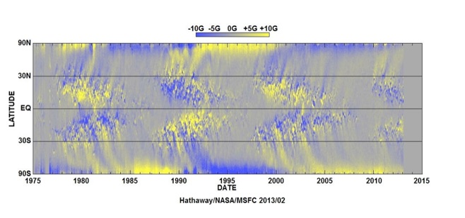
Sunspots on the solar surface are one manifestation of the solar activity cycle. They tend to appear at mid-latitudes in the beginning of the cycle and tend to occur at low latitudes towards the end. This pattern is believed to be connected to the underlying toroidal magnetic field, which migrates equatorward during the cycle, see Figure 5 for an illustration.
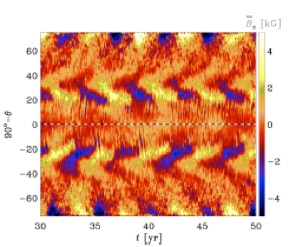
Global spherical shell simulations of convectively driven magnetic field generation could only produce poleward migrating or constant magnetic fields (e.g. Gilman 1983, Brun et al. 2004, Nelson et al. 2013). Just recently, my collaborators and I were able to reproduce for the first time solar--like equatorward migrating magnetic fields (Käpylä et al. 2012, 2013), see Figure 6 for an illustration. Later on, we could relate this equatorward migration to the negative radial shear present in the simulations (Warnecke et al. 2014) following a simplified magnetic field propagation model (Parker-Yoshimura Rule, see Parker 1955, Yoshimura 1975). It turns out that this rule can explain the propagation of magnetic
fields surprisingly accurately in a variety of global simulations of convection (Warnecke et al. 2016a; Käpylä et al. 2017). Just recently, we could quantify the validity of Parker-Yoshimura rule by determining all the relevant dynamo processes using the test-field method (Warnecke et al. 2018, Warnecke 2018). This result has important implications for the Sun: it constrains the region of magnetic field generation to the upper part of the convection zone, where the radial shear is negative.
Figure 5: Synoptic magnetogram of the solar magnetic field for the 3,5 cycles. It shows clearly the equatorward migration and polarity change of the magnetic field.
Figure 6: Solar-like equatorward migration of the magnetic field from a global simulation of magnetic field generation by convection in spherical shells. The toroidal magnetic field averaged over the azimuthal direction is shown as a function of latitude and time (Käpylä et al. 2012, 2013, Warnecke et al. 2014)
Formation of Sunspots
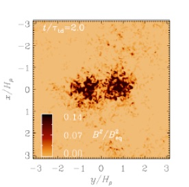
Sunspots on the solar surface appear to be dark, because a strong magnetic field suppresses the convective heat transport. Although high-resolution observations of sunspots exist for the solar surface, the process leading to their formation is still debated. In the most accepted theory, it is believed that flux tubes rise from inside the Sun to the surface generating bipolar regions of sunspots (e.g. Caligari et al.1995). This theory shows some difficulties and therefore alternative approaches have been developed, where flux concentrations are generated near the surface (Brandenburg et al. 2011, Stein & Nordlund 2012). One idea is that a hydromagnetic instability causes a spontaneous formation of sunspots. There, magnetic field suppresses locally turbulent pressure, leading to an inflow of material. These inflows drag along more magnetic fields, which then enhances the effect of suppressing the turbulent pressure. We were able to show that this effect can produce bipolar magnetic regions (Warnecke et al. 2013, 2016b, Losada et al. 2019). As seen in Figure 7, the two magnetic spots show some similarities to sunspots. These results have a large impact on the formation mechanism of sunspots and active regions as well as starspots.
Figure 7: Bipolar magnetic region. The normalized magnetic energy is shown at the corresponding surface. This illustrates the possibility to form bipolar magnetic flux concentrations by a turbulent hydromagnetic instability (Warnecke et al. 2013, 2015a).
Spoke--like Differential Rotation With a NEAR--SURface shear layer
The Sun is rotating differentially, the equator faster than the poles. Furthermore, the solar differential rotation profile shows conical contours of constant rotation rate (Figure 8), which has been known since the advent of helioseismology (Schou et al. 1998). This technique, where one identifies discrete wave modes on the surface of the Sun and inverts their properties, allows measuring the velocity and temperature distribution inside the convection zone with high precision. Mean-field models, where velocity fluctuations are parameterized by transport coefficients, could successfully reproduce the solar differential rotation (e.g. Kitchatinov & Rüdiger 1995). However, direct numerical simulations (DNS) of turbulent convection had to impose a latitudinal entropy gradient or a sub-adiabatic layer to obtain spoke--like differential rotation (e.g. Miesch et al. 2006, Brun et al. 2011). For the first time I was able to produce a spoke-like differential rotation pattern in DNS, which was generated self-consistently in a global model of turbulent convection with a coronal envelope (Warnecke et al 2013). Additionally, and for the first time theses simulations could also produce a near-surface shear layer at low latitudes, see Figure 9. This leads to the insight that the temperature structure at the surface is a very important ingredient to reproduce the correct rotation profile of the Sun (Warnecke al. 2016a). Additionally, the non-alignment of entropy and temperature gradients in the convection zone is responsible to achieve a non-cylindrical rotation profile. These results could confirm results from mean-field models and provide a new understanding of the generation of differential rotation in global convection simulations.
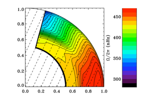
Figure 8: The internal differential rotation of the Sun as obtained from helioseismology.
The bottom of the convection zone lies at r = 0.713 solar radii. Image courtesy of GONG.
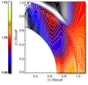
Figure 9: The internal differential rotation of a global spherical shell simulation of convective driven dynamo. The rotation rate is normalized by the mean rotation rate (Warnecke et al 2013).
Coronal ejection driven by magnetic field generation
The generation of magnetic fields and the ejection of magnetized plasma from the Sun have been separated research fields in solar physics. We made in Warnecke et al. (2010) an attempt to combine these fields of research driven by two main reasons:
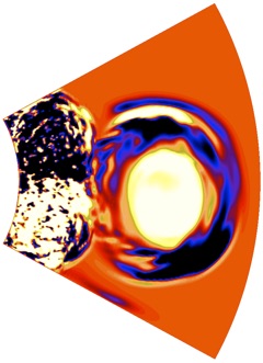
Firstly, for an effective production of magnetic field below the surface of the Sun, it is essential to transport magnetic helicity (dot product of magnetic vector potential and its magnetic field) to the surface and eventually out of the Sun. Coronal mass ejections are one promising way to do it (Blackman & Brandenburg 2003). Secondly, in the commonly used setup for modeling eruptions of coronal magnetic field and mass, an observed magnetic field and velocity configuration is taken for granted, neglecting underlying magnetic amplification mechanism, which actually generate these configurations. In Warnecke et al. (2010), we could already produce plasmoid ejections. With an improved model of Warnecke et al. (2011), we could generate self-consistent ejections, which have a similar shape than the observed solar coronal mass ejections, see Figure 10 for an illustration. In this simulation magnetic field gets ejected as a bipolar structure, in Figure 11 plotted as the current helicity density, which is a good proxy for helical magnetic at small scales. Later in Warnecke et al. (2012), we was able to generate ejections driven by convectively generated magnetic fields, where the structure and shape of the ejected material was similar to that of earlier simulations. This approach of combining the region below the solar surface, where the magnetic field is generated and the solar corona is an innovative idea, which led to important insights into the coupling of the convection zone and the outer atmosphere of the Sun.
See more here.
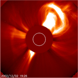
Figure 10: Coronal Mass Ejections (CME) observed by LASCO@ SOHO
Figure 11: Illustration of a coronal ejection of current helicity. Current helicity is the dot product of the magnetic field and its current density representing twisted magnetic field structures. On the left hand side of the plot, the solar convection zone has a negative sign (dark blue) of current helicity in the northern hemisphere and a positive sign (light yellow) in the southern hemisphere. The right hand side shows the neutral (orange) coronal extension containing a bi-helical ejection of current helicity (yellow and blue) (Warnecke et al. 2011).
Rotational dependency of stellar activity cycles
Many solar-like stars exhibit magnetic activity cycles similar as in the Sun. Analyzing the Mount Wilson chromospheric activity sample (Balinunas et al., 1995), Brandenburg et al. (1998) suggested that the cyclic stars fall on so-called inactive and active branches with positive slopes, when plotted as the ratio of rotation period and cycle period over rotational influence on convection in terms of Coriolis number or inverse Rossby number. This behavior is difficult to explain with dynamo theory. Moreover, I am involved in recent re-analysis of these data, which revealed that only the inactive branch seems to persist (Boro Saikia et al., 2018), which was also confirmed by Olspert et al. (2018). From numerical studies, we find no indication of these branches (Viviani et al., 2018, Warnecke, 2018) in agreement with Strugarek et al. (2017), see also Figure 2. However, we find that the axisymmetric cyclic magnetic field can be well explained with the Parker-Yoshimura dynamo wave (Warnecke, 2018) and that the non-axisymmetric cycle periods follow a different scaling than the axisymmetric ones (Viviani et al., 2018, Warnecke, 2018).
Figure 2: Composition of stellar cycles obtained from several numerical and observation studies showing ratio of rotation period and cycle period Prot/Pcycl over Coriolis number Co (Warnecke, 2018). All the numerical studies do not indicate stellar activity branches as suggested by Brandenburg et al. (1998) and Brandenburg et al. (2017).

Turbulent dynamo mechanism in stellar convection
Turbulent effects play an important role in the magnetic field generation of the Sun and stars. Unfortunately, current observations are not able to reveal these effects. One way to understand how these turbulent effects can generate magnetic field via dynamo mechanisms is to study global three dimensional magnetohydrodynamic simulation of the Sun and stars. There, the analysis tool „test-field method“ reveals turbulent transport coefficients as a parametrization of the turbulent effects and therefore let us get an idea of the dynamo mechanism operating in these simulations. The most prominent mechanisms are the α effect, turbulent pumping and the turbulent diffusion. Under my leadership, we applied the test-field method the for first time on such simulations (Warnecke et al. 2018). We find that the turbulent pumping is stronger than the meridional flow and therefore dominates the transport of magnetic field, see Figure 3. Furthermore, all transport coefficients show strong temporal variation with the magnetic cycle, indicating a non-linear saturation mechanism for the dynamo. Only if we are able to understand the dynamos operating in simulation, we can achieve conclusion about the magnetic field generation in the Sun and stars. We also used the test-field method to investigate the long-term magnetic field evolution similar to the Sun as found in Käpylä et al. (2016). We detect the reduction of part of the α effect and an enhancement of downward turbulent pumping during the event to confine some of the magnetic field at the bottom of the convection zone, where local maximum of magnetic energy is observed during the event (Gent et al. (2017) the same time, however, a quenching of the turbulent magnetic diffusivities is also observed.
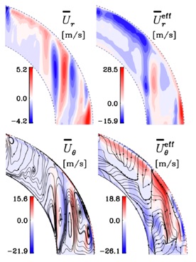
Figure 3: Effect of turbulent pumping on the transport of magnetic field. Ur and Uθ show the profile of meridional circulation without turbulent effects and Ureff and Uθeff shows the profile including the effect of turbulent pumping (Warnecke et al. 2018).
Non-force-free effects in coronal loops of the Sun
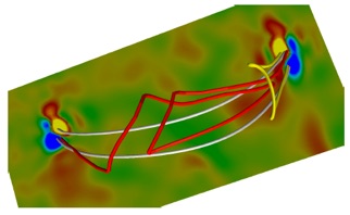
The solar corona is characterized by its high temperature and low plasma density. Mostly, there the magnetic field dominates the structures and dynamics of the coronal plasma as quantified by a low value of plasma-β. This is the ratio of gas and magnetic pressure. Under the assumption of a low-β corona, the magnetic field is often modeled using force-free extrapolation of the photospheric magnetic field (Wiegelmann et al., 2008). However, it turns out that the assumption of a low-β corona is not always valid and can lead to a wrong estimate of free magnetic energy and direction of currents above active regions (Peter et al. 2015). In a detailed study of a coronal loop above an emerging active region (Chen et al., 2015), we found that the total current along the emerging loop changes its sign from being antiparallel to parallel to the magnetic field (Warnecke et al., 2017). Around the loop the currents form a complex non-force-free helical structure, as shown in Figure 4. This is directly related to a bipolar current structure at the loop footpoints at the base of the corona and a local reduction of the background magnetic field (i.e. outside the loop) caused by the plasma flow into and along the loop. Furthermore, the locally reduced magnetic pressure in the loop allows it to sustain a higher density, which is crucial for the emission in extreme UV. Thus, the complex magnetic field and current system surrounding it can be modeled only in three-dimensional MHD models where the magnetic field has to balance the plasma pressure and it cannot always be determined correctly using a force-free extrapolation.
Figure 4: 3D rendering of the current and magnetic field lines around a corona loop above an emerging active region. The colored plane shows the vertical current at the base of the corona. The grey colored lines display the magnetic field lines connecting the positive and negative vertical current concentrations with each other, respectively. The red line shows a current line connecting the positive vertical current concentration on the right hand side to the negative concentration on the left-hand side. The yellow line shows also a current line, but connecting the positive and negative current concentrations on the right-hand side (Warnecke et al., 2017).
When observed in the extreme UV (EUV), the corona of the Sun above an active region is dominated by plasma loops over a range of temperatures from just below one million to several million Kelvin. The magnetic field in the corona channels the plasma and guides the energy flux. The first 3D models (Gudiksen & Nordlund, 2002, 2005a,b) created a loop-dominated corona; this confirmed the field-line braiding (Parker,1988) or flux-tube tectonics scenarios (Priest et al., 2002). The driving of the magnetic field in the photosphere in these models is prescribed by a photospheric velocity driver that mimics the solar granulation (Bingert & Peter, 2011, 2013). Here we use a data-driven 3D magnetohydrodynamic (MHD) model in which the observed (variable) magnetic field of an active region in the photosphere is considered as a lower boundary condition. We used non-Fourier heat flux evolution and semi-relativistic Boris correction to speed up the simulation significantly (see Chatterjee, 2019; Warnecke & Bingert, 2019). We can reproduce many aspects of the corona above an active region as shown in Figure 1. The emission that we synthesized from the model qualitatively reproduces the observed coronal features of this active region: long loops, fan-like loops, and small transient loops in the active region core. The structure of the observed photospheric magnetic field and its temporal evolution fully govern the appearance of the corona in an active region. Here the plasma is heated and forms EUV loops in the model at exactly the same place where they also appear in the real observations. The energy input in our model is solely based on the driving of the magnetic field and is thus very similar to the scenarios of field-line braiding and flux-tube tectonics scenarios. The success of our model therefore supports these
heating scenarios (Warnecke & Peter, 2019). A movie can be found here.
Data-driven models of the solar corona
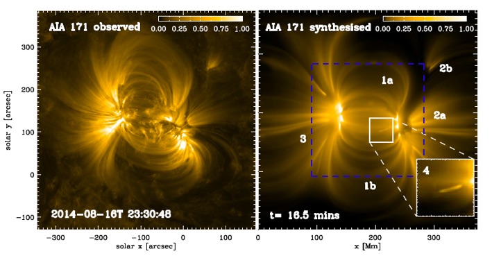
Figure 1: Comparison of observed emission and emission synthesized from model. The left panel shows the emission of the AIA 171 Å channel of AR 12139 on 16th of August 2014 at 23-30-48 UT near disk center. The right panel shows the synthesized emission of the same channel from the simulation as viewed from the top of the computation box. For better visibility, we use a non-linear scaling of the images (power of 0.7 for observation, of 0.4 for synthesized emission). The color bars reflect this. The peak value of counts in the observations (corresponding to 1.00) is 3500 DN/pixel, while this is a factor of six less for the model. This difference corresponds to a factor of 2.5 in density. The inlay shows zoom-in of the region indicated by the white square showing a compact small loop. There the color scaling is linear. The observations and the model cover the same physical space on the Sun with a FOV of (515.9 arcsec)2 corresponding to (374.4 Mm)2. The numbers and the blue dashed rectangle indicate features discussed in (Warnecke & Peter, 2019). A movie can be found here.