| Vector | Source | System | Units | X | Y | Z |
|
|
NSSDC | km | -135 927 895.1 | 126 880 660.0 | -340 567 928.0 | |
|
|
NSSDC | km/s | 18.54622396 | -8.287477214 | 2.89468231 | |
|
|
Tab.7 | km | -134 998 220 | -208 472 970 | -362 990 550 | |
|
|
Tab.7 | km/s | 18.624175 | -6.2275813 | 5.9890246 | |
|
|
Tab.7 | km | -134 998 220 | 125 262 330 | -341 329 890 | |
|
|
Tab.7 | km/s | 18.624175 | -8.0959913 | 3.0176330 | |
|
|
Tab.7 | km | -135 246 410 | 126 772 910 | -340 673 310 | |
|
|
Tab.7 | km/s | 18.546949 | -8.3037658 | 2.9273224 | |
|
|
SPICE | km | -135 922 227 | 126 877 772 | -340 564 861 | |
|
|
SPICE | km/s | 18.546466 | -8.287645 | 2.894987 | |
|
|
Tab.4 | km | 94 752 993 | -118 648 910 | -1 355 | |
|
|
Tab.4 | km/s | 22.792 | 18.478 | 0.00025 | |
| Tab.4 | km | 94 750 228 | -118 652 770 | -1 355 | ||
| Tab.4 | km/s | 22.802 | 18.471 | 0.00025 | ||
|
|
Tab.4 | AU | 0.633 3661 | -0.727 6925 | -0.315 5032 | |
|
|
AstrAlm | AU | 0.633 3616 | -0.727 6944 | -0.315 5035 |
Note that in the version of this paper published in Planetary&Space Science, 50, 217ff, the values calculated from Tab.4&7 are calculated for Jul 31, 1994 23:59 TT, not UTC.
The position and velocity vectors (state vector,
![]() in Tab.9) of the
Ulysses spacecraft which we used to determine the orbital
elements in Tab.7 was provided by NSSDC for
the Julian date
in Tab.9) of the
Ulysses spacecraft which we used to determine the orbital
elements in Tab.7 was provided by NSSDC for
the Julian date
![]() (Jul 31, 1994 23:59:00 UTC) in
heliocentric earth-equatorial coordinates for epoch
(Jul 31, 1994 23:59:00 UTC) in
heliocentric earth-equatorial coordinates for epoch
![]() .
.
In the following we describe how to derive the state vectors
for Ulysses and Earth from the orbital elements for this date
and compare the values with the respective data of the JPL SPICE system.
The Julian century for this date is
![]() (eqn.2).
From Tab.7 we take the values for the orbital
elements for Ulysses in
(eqn.2).
From Tab.7 we take the values for the orbital
elements for Ulysses in
![]() :
:
 |
(50) |
This position is in agreement with the ecliptic position available from
the spacecraft Situation Center for day 213, 1994:
![]() AU).
To compare this vector with the NSSDC value (
AU).
To compare this vector with the NSSDC value (
![]() ) we have first to transform from the ecliptic
) we have first to transform from the ecliptic
![]() system to the equatorial
system to the equatorial
![]() system using
system using
![]() .
Since
.
Since
![]() refers to the orientation of the Earth equator at
refers to the orientation of the Earth equator at
![]() we have to calculate the precession matrix using
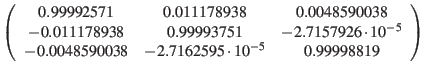
eqn.10 :
we have to calculate the precession matrix using
eqn.10 :
 |
(51) |
The distance to the original NSSDC position (
![]() ) is
697950 km (0.0046 AU), the difference in velocity 36 m/s in agreement with
the precision cited in Tab.7 for the orbital elements.
The respective position provided by the JPL SPICE system is (
) is
697950 km (0.0046 AU), the difference in velocity 36 m/s in agreement with
the precision cited in Tab.7 for the orbital elements.
The respective position provided by the JPL SPICE system is (
![]() ),
which deviates by 7062 km and 0.42 m/s from the NSSDC state vector.
),
which deviates by 7062 km and 0.42 m/s from the NSSDC state vector.
Now, we calculate the
![]() state vector of the Earth at the same time.
From Tab.4 we get the undisturbed orbital elements of the EMB:
state vector of the Earth at the same time.
From Tab.4 we get the undisturbed orbital elements of the EMB:
 |
(52) |
 |
(53) |
Using eqns.26 and 30 with
![]() (Tab.4),
we get the EMB state vector in
(Tab.4),
we get the EMB state vector in
![]() (
(
![]() ).
Given the low precision of the Ulysses position this would already be good enough
to get the geocentric Ulysses state vector but to compare with SPICE data or
the Astronomical Almanac we now apply eqn.32 to get the Earth state vector in
).
Given the low precision of the Ulysses position this would already be good enough
to get the geocentric Ulysses state vector but to compare with SPICE data or
the Astronomical Almanac we now apply eqn.32 to get the Earth state vector in
![]() (
(
![]() ), where we used the Delauney argument
), where we used the Delauney argument
![]() .
Finally we transform
from
.
Finally we transform
from
![]() to
to
![]() using
using
![]() as above to get
as above to get
![]() ,
which can be compared with the value given in section C22 of the Astronomical Almanac for 1994 (
,
which can be compared with the value given in section C22 of the Astronomical Almanac for 1994 (
![]() ,which
agrees with the value given by the SPICE system).
,which
agrees with the value given by the SPICE system).